Stage 6: Review, Reports, and Finalization
Overview
Stage 6 is where a person enters. The pipeline through Stage 5 produces an automatic spectral model with a complete audit record; Stage 6 turns that model into a finalized, reportable line list. It does two things: it applies human decisions to the automatic fit (adding a missed line, removing a spurious one, adjudicating a blend), and it consolidates and calibrates the final data products the reports present.
A human decision is not a cosmetic annotation. Every edit re-runs the fit for the affected window — a real nonlinear least-squares refit that updates the line frequencies, amplitudes, phases, and their covariance uncertainties — so the curated line list is as honestly fit as the automatic one. What a decision adds is provenance, not a physics prior: Stages 0–5 extract the best model the data support with no molecular-physics priors, and Stage 6 records whose decision produced each line. Model-as-prior fitting (fitting a molecular Hamiltonian to assign the lines) belongs to a separate program above this one; Stage 6 defines the data products and the decisions that program would build on.
Two CLI objects carry the stage, both mirrored on the Python interfaces. The ``review`` object builds the curation layer and applies edits; the ``report`` object renders the finalized record and never recomputes the fit. One distinction is worth fixing early, because it is easy to conflate:
``review run`` builds the worklist and the final-products table. It reads the existing fit and changes no peaks — it does not refit anything.
``review edit`` / ``merge`` / ``split``,
accept --candidate, and ``review apply`` are what refit: each applies a decision and re-runs the window’s least-squares fit in place.
Method
review run builds the curation layer over the Stage 5 fit: a single ranked
attention worklist of the windows that warrant a human look, and the
consolidated, calibrated final-products table the reports present. The analyst
works the worklist window by window, either editing it (which re-runs that
window’s fit) or accepting the automatic fit unchanged; either way the flag
clears. Every edit is appended to an anchored decision log that replays against
the file when an upstream stage is re-run, so curation survives re-analysis. Finally,
report renders the finalized record (the calibrated line table and a
self-contained HTML report), read-only. The sections below detail the flag model, the
worklist, the edit-and-refit verbs, the decision log, and the calibrated products.
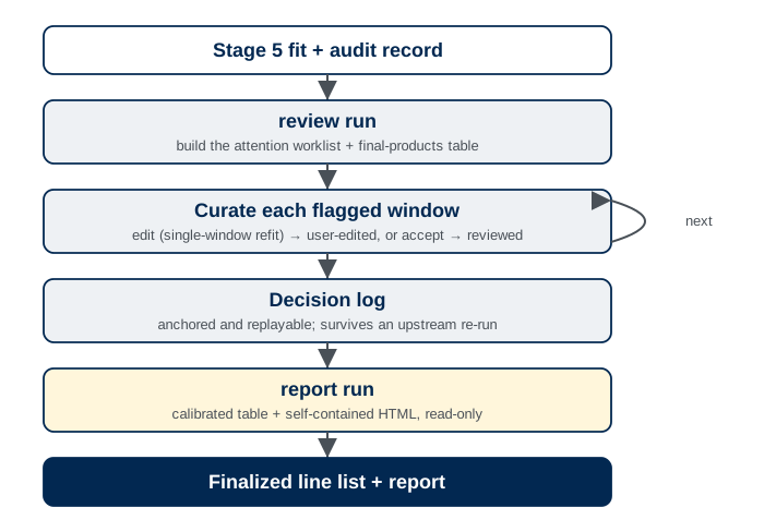
The Stage 6 curation loop. review run builds the worklist and the
final-products table; the analyst edits or accepts each flagged window (blue), each
edit re-running that window’s fit and logging an anchored, replayable decision;
report then renders the finalized record (gold), read-only.
Curation state and report-readiness
There is no global “finalize” action that freezes the record. Stage 6 is a curation layer over the Stage 5 fit, carrying two independent flags per window, shown as one combined label:
provenance —
auto(the fit produced it and no human has touched it),reviewed(a human looked and accepted the automatic fit unchanged), oruser-edited(a decision was applied);attention — none, or
needs-attentionwith one or more justified reasons. Attention is advisory: it never blocks a report. A window may legitimately stayauto · needs-attention.
The two axes are orthogonal. A window can be user-edited · needs-attention
(edited, but a neighboring spur still flags it) or user-edited with nothing left
to flag. Each peak additionally carries an origin of auto or user that
survives serialization, so a hand-added line is visibly marked wherever it appears.
Report-readiness is computed, not asserted. The only hard bar to generating a
report is a user-edited window whose decision has been invalidated by
re-running an upstream stage (see the decision log below).
needs-attention flags are reported honestly but never block.
Attention routing and the candidate ledger
review run builds one consolidated, ranked “needs attention” surface rather than a
scatter of per-feature lists, so the analyst has a single worklist. A window is
flagged for any of:
worst-ε — the window’s reduced \(\chi^2\) fails the signal-to-noise-aware acceptance gate (the same standard
fit checkuses);over-split — a sub-resolution pair was auto-merged, or a member’s amplitude variance-inflation factor flags a degenerate split for the analyst to confirm;
candidate-bearing — the candidate ledger (below) holds a revivable rejected line with strong residual evidence (gated by a stiffer bar than the display ledger, so the surface stays actionable);
spur-adjacent — a fitted line sits next to a masked clock/LO spur;
edge/boundary — a line sits at a window edge, where leakage coupling is hardest.
A flag clears one of two ways: an edit (the window becomes user-edited) or an
explicit review accept (the window becomes reviewed, recording that a human
looked and was satisfied). Routing never forces a resolution; there is no
rubber-stamp. review rank --by <metric> re-sorts the whole worklist worst-first by
a chosen diagnostic (min-snr, max-vif, chi2r, candidate-evidence,
edge-distance, spur-proximity, or merged-chi2r).
The candidate-bearing flag draws from a candidate ledger that Stage 6 derives, on
demand, from data the Stage 5 fit already persisted. Every line the fit considered
and rejected survives in the per-window audit trail and rescue history; the ledger
collects the add-loop rejects, the rescue candidates, the failed blend-split trials,
and the separation rejects, and normalizes them to one entry per distinct molecular
frequency (deduplicated across rescue rounds). Each entry carries its best evidence
seen, its rejection reasons, and the recorded seed needed to revive it. A display
bar keeps gate-killed dust off the worklist, so only candidates with real residual or
rescue evidence surface. Because the ledger is a pure function of the persisted Stage 5
data, review show --candidates renders it without re-fitting; it is the menu the
analyst draws from when a window is flagged candidate-bearing.
Editing the fit
Every edit verb refits the edited window and propagates into its dependents. The
edited window re-seeds from its own persisted state (its fitted peaks as seeds, its
frozen contributors reconstructed from its own record), applies the add or remove, runs
one joint nonlinear least-squares fit with the production fitting primitive, and replaces
that window’s entry in the stored fit. Because a strong line contributes its frozen
leakage skirt to neighboring windows, the edit then cascades: every window that froze
a skirt from the edited one has its frozen background rebuilt from the edited window’s
current fit and is refit, in dependency order, so the file never carries a neighbor’s
stale model of an edited line. The cascade refits are fit-only — no conservative
discovery, no rescue, no Stage 4 renegotiation — and are a deterministic consequence of
the edit rather than logged decisions of their own. The propagation is usually far below
the reported precision: a split or merge that preserves a line’s total power and centroid
leaves its far-field skirt unchanged, so most edits move their dependents by
\(\ll\sigma_f\), and the case that matters is an edit that changes a strong line’s
amplitude or position by a large amount. (Contrast review run, which builds the
worklist and products but refits nothing.)
review edit --window N --add F/--remove F— add or remove a line.--addsnaps to the nearest ledger candidate within tolerance (reviving its recorded seed) or seeds a fresh line atF;--removesnaps to the nearest fitted peak. Both flags repeat, and a run of adds and removes on one window resolves into one refit.review merge --window N --peaks F1,F2— collapse a set of lines to one (amplitudes summed, frequency the signal-to-noise-weighted mean). When the set matches a pair for which the observation-only doublet pass already recorded a merged-single alternative,mergesnaps to that recorded seed.review split --window N --peak F [--into K]— replace one line withK(default 2) straddlingFby a fraction of a resolution element.review accept --window N— the “looked, no change” dismissal (the window becomesreviewed); the fit is untouched. With--candidate Fit instead revives a ledger candidate, which does refit.
merge and split are physics-aware-reseed sugar over add-plus-remove. All edits
carry user provenance.
A user edit bypasses the accept gate but not the optimizer. The analyst is the gate: a user-added line is kept without the F-test the automatic loop applies. It still faces the fit honestly, though — if the optimizer drives it to zero amplitude or collapses it onto a neighbor, the result reports that rather than keeping a phantom. Subsequent automatic passes are bound to the decision: the survival prune, the merge cleanup, and the rescue pass will not prune a user-added line nor re-add a user-removed one, because either would make the verb feel broken.
Every edit appends an entry to an ordered decision log persisted in the file, so
the .ftmw reproduces the curated analysis with no side channel. Each entry is
anchored to a window identity and a molecular frequency, and records its kind, its
user provenance, and an evidence snapshot. review log lists the history;
review undo reverts the most recent decisions by restoring the snapshotted
automatic fit and replaying the surviving decisions on top.
Because the decisions are anchored rather than baked in, re-running an upstream stage
does not silently discard them. Replay re-applies each decision wherever its anchor
still resolves — refitting the window just as the original edit did — and surfaces a
comparison (reduced \(\chi^2\) with and without the decision, the peak-count and
frequency deltas) so the analyst can decide whether to revisit it. A decision is
invalidated only when its anchor no longer resolves: the window is gone, or the
frequency has fallen out of any window or out of band. An invalidated user-edited
window is the sole hard bar to report generation; the report, when generated, logs the
Stage 6 decisions for honesty. Throughout, the curated result stays separable from the
automatic one, so a curated fixture never silently masquerades as an automatic
benchmark.
Final products and the frequency budget
review run consolidates the final-products table: the single, calibrated line
list the reports present, persisted in the file and rebuilt after every edit so it is
never stale. Each row is one accepted line, carrying its calibrated and raw
frequencies, the amplitude, phase, and signal-to-noise with their uncertainties, the
three-term frequency budget, the originating window, the origin provenance, and any
clock-lattice flag. The exact columns are listed under
the table output below.
The frequency uncertainty is composed as three independent terms in quadrature:
\(\sigma_\text{stat}\) is the statistical precision from the fit covariance, the per-line frequency error Stage 5 reports.
\(\sigma_\varepsilon\, f_\text{baseband}\) is the timebase-calibration residual: a fractional digitizer-clock scale error \(\varepsilon\) multiplies the line’s baseband offset from the probe, so it grows with distance from the local oscillator. It is zero unless self-calibration ran.
\(\sigma_\text{floor}\) is a user-settable systematic floor (
review run --sigma-floor, default0kHz), the home for an instrument’s irreducible run-to-run accuracy term that the clock lattice cannot pin. The default of zero keeps the reported budget honest about precision and leaves any accuracy claim to the analyst who knows the instrument.
Calibration is a reported state, never a report gate. Whether the frequency axis needs self-calibration is a property of the instrument’s clock reference, declared alongside the clock tree, and defaulting to “assume the axis is absolutely calibrated” when nothing says otherwise. The table and the report state one of three cases plainly:
Rb-locked (declared, or the default) — the axis is absolutely calibrated by a frequency standard; \(\varepsilon \equiv 0\) and self-calibration is a null operation. Frequencies are trusted as-is.
Free-running, self-calibrated —
timebase_calibrationran; the measured \(\varepsilon\) is applied and its residual folded into the budget.Free-running, not self-calibrated — frequencies are reported uncalibrated with a strong recommendation to self-calibrate.
The timebase self-calibration handles exactly one topology: all signal-chain clocks
locked, with the digitizer the single free-running source, whose fractional scale
error it fits from how the locked spurs appear to drift. A declaration outside that
topology (a locked digitizer with some other free-running clock) reports as
free-running with self-cal unavailable rather than producing a wrong
\(\varepsilon\). This is a stated limitation, not a gap to be filled in this layer,
so timebase_calibration is a soft input: strongly recommended for a declared
free-running instrument, a null op for a locked one, and never a hard bar to a report.
Each line in the report and the per-window detail also carries the per-line ``qual``
determinacy score introduced in Stage 5 — how many of four
independent checks the line clearly passes, written k/4 (detected with margin,
amplitude identifiable, position pinned, isolated). It also serves as a review rank
--by key. The framing is the same here: it measures how firmly the data determine a
line, not whether the line is a real, assignable transition. A high score can still
attach to an unmasked spur or an unassigned feature, so it informs curation rather than
gating it.
Catalog cross-reference
Every report level accepts an optional --catalog of expected frequencies. For each
reported line the report flags the nearest catalog entry within a geometric tolerance
\(N\sqrt{\sigma_f^2 + \sigma_\text{cat}^2}\) (--catalog-nsigma, default 3)
and echoes its opaque label — proximity annotation only, never an assignment. The
pipeline emits unassigned lines; the cross-reference is a cross-check, never a fit
input. The reader accepts a CSV/whitespace table (frequency_mhz plus an optional
uncertainty and label, with the uncertainty unit read from the header) and the
Pickett/SPCAT .cat predicted-line catalog.
A catalog also unlocks the pull calibration: the distribution of \((f_\text{fit} - f_\text{cat}) / \sigma_f\), which should be a unit normal when the \(\sigma_f\) budget is honest. The report summarizes the pull (mean, spread) and flags a spread much greater than one (an optimistic budget) or much less than one (a conservative one). It validates the budget; it is not a shipped gate.
Running the stage
Stage 6 requires Stage 5; the timebase calibration is a soft
input. review run builds the curation layer and the final-products table in one
pass, printing a summary of the worklist and the calibration state:
$ ftmwpipeline review run exp_2638.ftmw
review run: 277 window(s), 5 needing attention
  candidate-bearing: 3
  over-split: 1
  spur-adjacent: 1
final products: 638 peak(s), calibration Rb-locked (eps=±0.000 ppm), sigma_floor=0.000 kHz

$ ftmwpipeline review rank --by chi2r --top 3 exp_2638.ftmw
$ ftmwpipeline review edit --window 217 --add 31214.20 exp_2638.ftmw   # refits window 217
$ ftmwpipeline report run exp_2638.ftmw --output-dir report/
report run: wrote table to report/exp_2638_lines.csv
report run: wrote self-contained full HTML report to report/exp_2638_report.html
The same operations on the Python interfaces, with the values each call returns:
import ftmwpipeline.api as ftmw

result = ftmw.review_run("exp_2638.ftmw")
print(result.n_windows, result.n_attention)        # -> 277 5
print(result.reason_counts)                         # -> {'candidate-bearing': 3, ...}

for w in ftmw.rank_windows("exp_2638.ftmw", by="chi2r", top=3):
    print(w.window_id, w.metric, round(w.value, 2), w.n_peaks)
# 217 chi2r 3.81 2
# 49  chi2r 2.94 5
# 188 chi2r 2.40 1

edit = ftmw.review_edit("exp_2638.ftmw", window_id=217, add=[31214.20])
print(edit.n_peaks_before, edit.n_peaks_after, round(edit.chi2r_after, 2))   # -> 2 3 1.18

paths = ftmw.report_run("exp_2638.ftmw", output_dir="report/")
print(paths)   # -> {'table': 'report/exp_2638_lines.csv', 'html': 'report/exp_2638_report.html'}

# or, object-oriented
from ftmwpipeline import Pipeline
pipe = Pipeline.open("exp_2638.ftmw")
pipe.review_run()
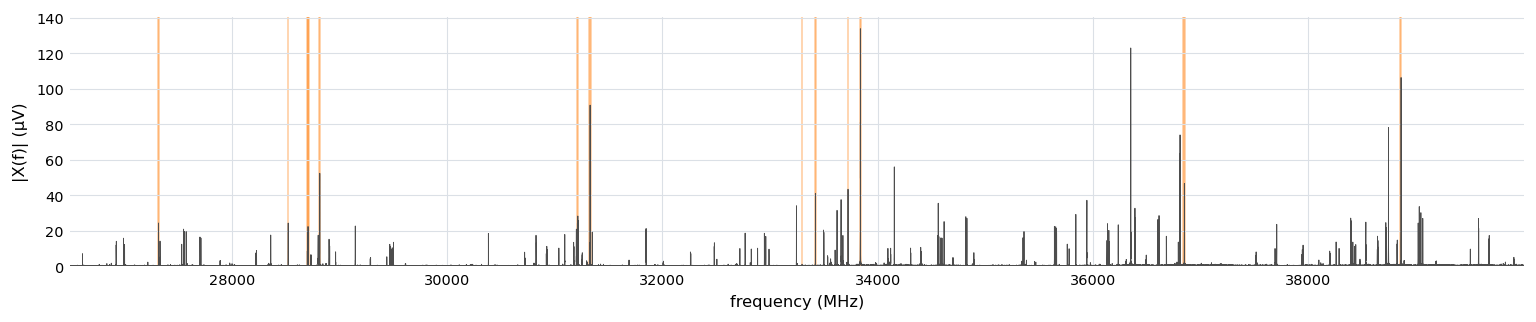
The Stage 6 review surface over the example experiment: the report’s full-spectrum
index overview. The finalized active spectrum (magnitude) runs across the whole
band, with the windows the review flagged for attention shaded — the analyst’s
worklist at a glance. The bulk of the spectrum is settled auto model; attention
is drawn only to the few windows where a close call, a candidate, or an
edge-coherent residual warrants a human look.
Reports
The report object renders the finalized record into an output directory (the
current directory by default); it never recomputes the fit.
report table exports the final-products table on its own as CSV, JSON, or LaTeX
(--format; the LaTeX form is a booktabs table for a paper’s supplementary
material). Spectroscopic fitting formats (Pickett .lin / SPFIT) are out of scope by
design, because the pipeline emits unassigned lines. The CSV is the canonical form: a
commented provenance header followed by one row per accepted line. Its columns, in
order, are frequency_mhz (calibrated), sigma_f_khz (the total budget), its
three components sigma_stat_khz / sigma_eps_khz / sigma_floor_khz,
frequency_raw_mhz (uncalibrated) and f_baseband_mhz, amplitude /
amplitude_err (in a header-declared unit), phase_rad / phase_err_rad,
snr / snr_err, origin, window_id, and clock_lattice. With
--catalog four columns append: catalog_label, catalog_freq_mhz,
catalog_delta_khz, and catalog_pull. A representative excerpt:
# experiment: exp_2638
# calibration_state: rb_locked
# epsilon_ppm: 0.000
# sigma_floor_khz: 0.000
# probe_freq_mhz: 26000.000
# sideband: upper
# amplitude_unit: uV
# n_peaks: 638
frequency_mhz,sigma_f_khz,sigma_stat_khz,sigma_eps_khz,sigma_floor_khz,frequency_raw_mhz,f_baseband_mhz,amplitude,amplitude_err,phase_rad,phase_err_rad,snr,snr_err,origin,window_id,clock_lattice
36350.112100,0.42,0.42,0.000,0.000,36350.112100,10350.112100,18.3,0.37,0.31,0.02,210.4,4.2,auto,217,
36389.044700,0.55,0.55,0.000,0.000,36389.044700,10389.044700,9.1,0.41,-1.12,0.05,71.6,3.2,auto,218,
report run is the default deliverable: it writes that table (<stem>_lines.csv by
default) and a self-contained HTML report (<stem>_report.html), one portable
file with the stylesheet inlined and every figure embedded. The report opens
read-only, with an opt-in Curate toggle that collects edits in the browser and
exports them as a curation file for review apply to replay. Its anatomy, the
in-browser curation cart, and the curation-file language are documented on the
Fit Curation page.
report diff is a before/after review aid for vetting a curation before
committing to it. It writes a self-contained <stem>_diff.html that compares the
automatic fit with the current curated fit, side by side, for every window the
curation changed materially — both the windows edited directly and the dependents the
contributor-edit cascade touched — so the changes can be
reviewed in one place without maintaining and diffing two separate files. Each window
shows its before and after \(|X|\)-and-model panels (click either to zoom) with a
stat line giving the change in reduced \(\chi^2\), the shape-error fraction, and the
peak count; a window is included when a peak was added or removed, a peak moved
appreciably, or the fit quality shifted beyond a small threshold, which filters out the
sub-noise cascade jitter. The comparison is possible because the first curation edit
snapshots the automatic fit inside the file; before any edit (nothing to compare) the
report says so. Like the other report verbs it is read-only and never recomputes the
fit.
Limitations
The cascade is least-squares only. Propagating an edit refits each dependent against the corrected skirt with the production primitive, but does not re-run line discovery or rescue on it: it re-determines a dependent’s existing lines, and will not add a line that the corrected background newly reveals. A dependent that a large edit leaves visibly under- or over-fit (its reduced \(\chi^2\) is the tell) is curated directly, which is consistent with the model — it becomes a directly-edited window.
Curation is recorded, not interpreted. The decisions and their provenance persist, but adjudicating a genuine sub-resolution doublet against an over-split remains the analyst’s call, supported by the observation-only doublet statistics and a catalog where one exists.
Precision, not accuracy, unless self-calibration ran. The reported budget carries the formal precision plus whatever calibration the declared clock tree supports. An undeclared systematic offset is left to
--sigma-floor, not invented by the pipeline.
With the line list reviewed, calibrated, and finalized, the report renders the analysis a reader can trust: the line positions, their uncertainty budget, and the provenance of every decision that produced them.