Stage 5: Peak Fitting

Overview

Stage 5 turns the Stage 4 window plan into the fitted line list: for every line it recovers a frequency, an amplitude, a phase, and a decay time, each with an uncertainty, by fitting a finite-acquisition line-shape model to the complex spectrum window by window. This is where the spectroscopic numbers (the line positions a catalog is built from) actually come out.

The fit is deliberately conservative. Rather than fit a fixed number of lines per window, it grows each window’s model one line at a time and keeps a new line only when the data demand it on a formal statistical test. Everything that makes a real instrument’s spectrum hard (truncation leakage, blended lines, clock spurs, under-modeled skirt wings) is handled by an explicit mechanism rather than by smoothing it away, so the reported parameters and their uncertainties stay trustworthy.

Method

Stage 5 fits each window of the Stage 4 plan independently, seeding the lines Stage 3 detected robustly and then growing the window’s model one line at a time, keeping each added line only when a formal test demands it. A window is seeded with its Stage 3 primary detections; the add-one-peak loop then proposes the next residual peak from the weak-line candidates and accepts it only when its fit improvement clears a window-size-independent penalty bar, stopping when no candidate clears it. A leakage-wing baseline is added where the residual stays coherent, a rescue pass recovers weak lines the loop missed, and a renegotiation with Stage 4 thaws a frozen contributor or merges windows when a coherent edge remains. As each window converges it is cleaned in place — lines below the detection floor pruned, sub-resolution pairs the fit cannot justify merged — before the dependency-ordered parallel batches release the windows that depend on it, so every window reads clean, current neighbors. The model the fit uses, and the frame it runs in, come first; each mechanism is then taken in turn.

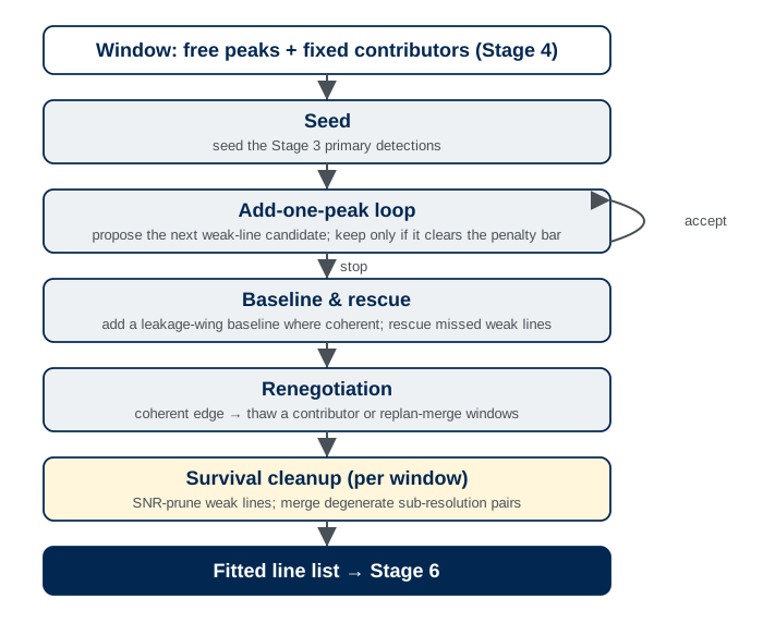
The Stage 5 fit lifecycle. Each window (blue) is seeded with its Stage 3 primary detections, grown by the add-one-peak loop (which iterates while a proposed line clears the penalty bar), then refined by the baseline, rescue, and renegotiation steps, and cleaned in place (gold) — pruned and merged — before the window is released. The windows run in dependency-ordered batches, so each reads clean, current neighbors.

Line-shape model

A molecular line in an FTMW experiment is an exponentially damped cosine, excited at the active-region turn-on and observed over a finite acquisition of length \(T\). Its complex Fourier transform is not a Lorentzian: the finite observation window wraps every line in a coherent truncation-leakage skirt, a sinc-like ripple that reaches tens of megahertz from the line center. Stage 5 fits the exact finite-\(T\) response rather than fighting the leakage with apodization (which would broaden the lines and bias the shape, and is why the active FT is left unwindowed).

Each line in a window carries three free parameters: an amplitude \(A\), a baseband frequency offset \(\Delta f\) (MHz) from the window reference, and a phase \(\varphi\). All lines in the window additionally share one decay time, rather than fitting it per line (Shared decay time covers when it is free and when it is held). For the default Lorentzian envelope \(e^{-t/\tau}\), one line’s modeled response is

\[X(\Delta f) \approx \tfrac{1}{2} A\, e^{i\varphi}\, h_T(\Delta f; \tau), \qquad h_T(\Delta f; \tau) = \frac{1 - \exp\!\bigl[-(1/\tau + i\,2\pi\,\Delta f)\,T\bigr]} {1/\tau + i\,2\pi\,\Delta f},\]

the exact finite-\(T\) transform of a damped cosine observed over \([0, T]\). At line center \(h_T(0) = \tau_\text{eff} = \tau\,(1 - e^{-T/\tau})\), and far from center its magnitude falls off as the \(1/|\Delta f|\) truncation-leakage skirt with a definite, coherent phase. Because the model carries that skirt exactly, a strong line’s leakage can be subtracted from a neighboring window exactly — which is the entire basis of the Stage 4 fixed-contributor scheme.

The Gaussian alternative replaces the exponential envelope with \(e^{-(t/\tau_G)^2}\), for instruments whose lines relax with a Gaussian profile. Its finite-\(T\) response is the closed-form complex transform

\[h_T(\Delta f; \tau_G) = \frac{\sqrt{\pi}}{2}\,\tau_G\, e^{\beta^2} \bigl[\operatorname{erf}(T/\tau_G + \beta) - \operatorname{erf}(\beta)\bigr], \qquad \beta \equiv i\,\pi\,\tau_G\,\Delta f,\]

carrying the same \(\tfrac{1}{2} A\, e^{i\varphi}\) amplitude–phase prefactor and the same window-shared decay time (now \(\tau_G\)). Its real prefactor \(e^{\beta^2} = e^{-\pi^2\tau_G^2\,\Delta f^2}\) is the Gaussian line core, and at center \(h_T(0; \tau_G) = \tfrac{\sqrt{\pi}}{2}\,\tau_G\operatorname{erf}(T/\tau_G) = \tau_{\text{eff},G}\). The envelope shape is normally not set by hand — the Stage 2b line-shape vote recommends it, and the fit consumes the matching decay-time calibration (\(\tau\) or \(\tau_G\)).

Putting the terms together, the complete model of a window on its baseband-offset grid \(u\) (MHz from the window reference) is

\[M(u) = \underbrace{\sum_{j\,\in\,\text{free}} \tfrac{1}{2} A_j\, e^{i\varphi_j}\, h_T(u - \delta_j;\, \tau)}_{\text{free peaks (fitted)}} \;+\; \underbrace{\sum_{c\,\in\,\text{fixed}} \tfrac{1}{2} A_c\, e^{i\varphi_c}\, h_T(u - \delta_c;\, \tau_c)}_{\text{fixed contributors (frozen)}} \;+\; \underbrace{B(u)}_{\text{baseline}}.\]

Each free peak contributes three fitted parameters (amplitude \(A_j\), offset \(\delta_j\), and phase \(\varphi_j\)), and all free peaks share the single decay time \(\tau\) (fitted or held, per Shared decay time). Each fixed contributor \(c\) is frozen at the parameters from its own window’s fit (amplitude, offset, phase, and its own decay time \(\tau_c\)) and only adds its leakage skirt here, never a free line. \(B(u)\) is a low-order complex baseline polynomial, present only when the leakage-wing trigger fires (Leakage coupling between windows). The same form holds for the Gaussian envelope, with \(h_T\) the Gaussian response and \(\tau_G\) in place of \(\tau\).

The fit runs on the active-portion FT — the transform of just the active FID samples, the same surface Stage 2 measured its noise on, already in the \([0, T]\) form the model expects. Each window is sliced from the active FT and its molecular-frequency grid is converted to a small signed baseband offset about the window reference: a line near 36 GHz is fit as a ~MHz offset, not as an absolute ~36 GHz number. The sideband sign relating molecular and baseband frequency is taken from the experiment metadata; the opposite sign would conjugate every leakage skirt and bias the fitted frequencies while leaving the magnitude residual looking plausible.

Conservative add-one-peak loop

Each window is fit by seeding the lines Stage 3 detected robustly, then growing the model one line at a time over the remaining candidates:

1. Seed the primaries. Stage 3’s primary (Blackman–Harris) detections are the robust strong-line positions, so Stage 5 trusts them and seeds them all up front. In a window with several, each is placed in turn against the running residual — so a dense cluster converges on its lines instead of collapsing onto one basin — and the seeded set is then fit jointly (amplitude, frequency, phase, and, where eligible, the shared decay time) by complex nonlinear least squares against the window’s data, weighted by the Stage 2 per-bin noise. A window with one primary is seeded with that line.

2. Propose. From the gap candidates — the weak lines the Stage 3 matched-filter pass nominated between the strong ones — pick the strongest in the current residual that has not yet been tried and trial-fit it jointly with the lines already accepted. The robust primaries are not re-adjudicated by the gate; only these weak candidates are.

3. Accept or stop. Keep the new line only when its chi-squared improvement clears a fixed penalized bar: the drop \(\Delta\chi^2\) from adding the line must exceed \(2\lambda\,\Delta k\), where \(\Delta k\) is the parameters the line costs and \(\lambda\) is a single global strictness (a stricter, BIC-like setting of the textbook information criterion). Because the two models compared share the window’s bins, \(\Delta\chi^2\) is the local evidence for the line and the bar carries no window geometry — so a window padded with quiet noise cannot manufacture significance for an extra line. The chi-squared is scored against a per-bin noise inflated by the lineshape-fidelity budget where the model is bright, so a candidate that only absorbs a strong line’s irreducible shape misfit cannot clear the bar. A candidate that fails is rejected, and the loop stops after a bounded run of consecutive rejections, when no candidate remains, or when a width or separation bound is reached.

Because the residual is weighted by the real per-bin noise, a converged window sits at its noise-and-fidelity floor, and the window-size-independent bar keeps the gate honest — the loop adds a line only on genuine local evidence, not to chase a lineshape floor or to exploit a window’s quiet bins. A classical F-test on the \(\chi^2\) drop is recorded at each step as a familiar diagnostic, but it does not gate acceptance. The derivation of the gate, the window-size bias it avoids, and its cross-instrument validation are in the fitting-statistics methods note.

Blend-aware seeding. A single line fit to a close blend lands at the blend’s centroid and leaves an elevated reduced \(\chi^2\). When that happens the seeder retries with two (then up to three) lines straddling the feature rather than stacked at the drifted centroid, which recovers blends down to about half a line width apart. This blend escalation, not a large patience budget, is what makes the conservative loop resolve real doublets.

Shared decay time

All lines in a window share one decay time — a single physical relaxation governs the whole local spectrum, and sharing it keeps the fit well determined. Whether that decay time is a free parameter depends on how much signal the window carries:

• A window whose strongest line clears the free-\(\tau\) floor (fit_tau_min_snr, default SNR 10) fits \(\tau\) freely, bounded to a band around the Stage 2b majority value \(\tau_\text{maj}\) and softly anchored there by a penalty so it cannot run away.

• A weaker window holds \(\tau\) fixed at \(\tau_\text{maj}\) (the band-local value when per-band calibration is available, otherwise the band-wide value, otherwise \(T/3\)). A faint window cannot determine its own decay time, so it borrows the calibrated one rather than letting \(\tau\) absorb noise.

The penalty is a soft bidirectional prior centered on \(\tau_\text{maj}\) with a width set by the Stage 2b uncertainty \(\sigma_\tau\); it matters most for the Gaussian shape, where an unconstrained \(\tau_G\) can trade against the baseline.

Leakage coupling between windows

A window is not fit in isolation. The truncation-leakage skirt of every strong line reaches well beyond its own window, so each window must account for the leakage of its neighbors, absorb the residue the discrete model cannot capture, and, when coupling only surfaces once the lines are fit, renegotiate its boundaries with Stage 4.

Fixed contributors and the fit order. A window does not fit the strong lines that live in other windows, but it must still account for their leakage reaching into its band. Stage 4 attaches each such line as a fixed contributor: its damped-cosine term, with parameters frozen at the values from its own fit, is evaluated in this window’s model (it is added to the model, never subtracted from the data, consistent with the least-squares contract). A contributor whose own signal-to-noise is too low to freeze confidently is flagged for the thaw handshake below. Because a frozen skirt can only be drawn once its source line has been fit, windows carry a dependency order: Stage 4 groups them into parallel batches (batch 0 has no dependencies, batch 1 depends only on batch 0, and so on), and Stage 5 fits them concurrently across a worker pool, releasing each window as soon as the windows it depends on have converged. The result is identical to a strictly sequential fit; parallelism only shortens the wall-clock time (see performance).

Leakage-wing baseline. Hundreds of distant lines each contribute a little coherent leakage that the discrete fixed-contributor set cannot fully represent, and a single strong neighbor’s skirt is never modeled perfectly. The residue is a smooth, coherent pedestal under a window — not a narrow line, but enough to inflate \(\chi^2\) and bias the lines sitting on it. Stage 5 absorbs it with an evidence-triggered baseline: a low-order complex polynomial added to the window’s model. It fires only where the evidence calls for it — when the residual at a window edge is still coherent (the edge-coherence statistic exceeds edge_threshold) or when a low-order polynomial explains a smooth in-band residual on an F-test (smooth_threshold). When it fires, the window is refit with the baseline and a re-freed \(\tau\), so the added flexibility is priced into the per-line uncertainties. The default order (4) follows a pedestal’s gentle ramp and curvature while remaining far too smooth to mimic a real line (every window spans many bins), and the F-test trigger is the guardrail against over-fitting.

Renegotiation with Stage 4. Some coupling is only visible once the lines are fit. After a window converges, Stage 5 checks whether its edges still carry coherent residual leakage, and if so it renegotiates rather than shipping an under-fit window:

• Thaw. When a fixed contributor is responsible (its frozen parameters no longer explain the boundary, or it was flagged not freeze-eligible), the contributor is unfrozen and co-fit jointly with the dependent window. This does not fit the line a second time: its single free fit is reopened and re-determined jointly across the coupled windows, replacing the frozen copy rather than adding another. It is the common, cheap case (the reference experiment’s 36350/36389 MHz pair, each the other’s contributor, resolves this way).

• Structural replan. When no contributor accounts for the coherent edge, because a real line straddles the boundary, Stage 5 asks Stage 4 to merge the two windows through its re-plan entry point, bumping the plan revision, and refits the affected batches.

Both are bounded by round caps for guaranteed termination, and every attempt, accepted or not, is recorded in the fit’s audit trail. A window split is deliberately not part of the handshake; over-fitting is handled after the fact by the survival pass below.

Refining the line list

Three mechanisms shape the final line population: recovering real lines the initial pass missed, excluding instrumental artifacts, and pruning lines the data do not support.

Residual rescue. After the add loop converges, a rescue pass re-examines the residual for weak lines the initial nomination missed — typically lines on the shoulder of a strong neighbor, where the Stage 3 position was slightly off. It nominates generously from residual prominence and then gates each candidate through the same penalized acceptance the main loop uses, with a remove-and-refit cleanup that drops any line the joint fit no longer supports and merges sub-resolution duplicates. Rescue is bounded by a round cap and is what closes the gap between detection and a complete fit on dense, high-dynamic-range spectra.

Final add-from-convergence. Once a window has fully converged and been cleaned, a last recovery pass revisits the strongest peaks its residual still carries. For each it attempts a single line addition warm-started from the converged fit — the existing lines held at their fitted positions, the new line seeded exactly at the residual peak — through the same penalized acceptance gate and minimum-separation guard the main loop uses. Seeding from convergence at the true residual location recovers a close companion, a weak line about one and a half resolution elements from a moderate neighbor, that the mid-fit nomination loses when its symmetric trial seed collapses the pair; the unchanged gate still rejects a genuine over-split, so the pass adds recall without adding overfit risk. A candidate that sits inside a brighter line’s lineshape-error shadow — residual signal that scales with the neighbor’s brightness rather than marking a separate molecule — is skipped, so a strong line’s imperfect-shape sidelobe is never promoted to a phantom detection. The residual signal-to-noise that triggers an attempt is final_add_snr_threshold (10); set it to 0 to disable the pass.

Spur masking. Clock and local-oscillator harmonics appear as spurs: persistent continuous-wave tones that sit at integer megahertz and are a single bin wide — narrower than any finite-\(T\) line shape can be. Fitting one as a molecular line would manufacture a spurious detection. Stage 5 identifies a spur by combining an integer-megahertz position with either a frequency-domain narrowness test or the Stage 2b flat/saturated catalog, and excludes the masked bins from peak nomination and from the \(\chi^2\) / residual sums. A declared instrument clock tree sharpens this: the locked-clock intermodulation lattice replaces the bare integer-megahertz anchor, and a drifting-tone lane handles a free-running digitizer clock.

Survival cleanup. Four automatic cuts run on each window in place as it converges, before the dependency-ordered batches release the windows that depend on it — so a dependent always freezes a clean, current background. All leave hand-added (user-origin) lines untouched.

• Signal-to-noise prune. Every automatically fitted line whose post-fit SNR falls below the survival floor is dropped, windows left empty are removed, and partially pruned windows are refit so the survivors’ parameters stay honest. The floor tracks the Stage 3 promotion cutoff: by default it is that cutoff scaled by snr_survival_factor (1.1), so a survivor never sits below the signal-to-noise that admitted the line at detection, and raising the Stage 3 cutoff raises the survival bar in step. Setting snr_survival_floor pins an absolute floor instead. The prune iterates to a fixed point, because removing a line and refitting can push a marginal neighbor below the floor.

• Degenerate-pair merge. A sub-resolution pair that the fit split into two lines is merged back into one when a member’s amplitude is statistically unidentifiable. Two criteria trigger the merge, both within the separation guard: the amplitude variance-inflation factor \(\text{VIF} = (\sigma_A / A)\cdot\text{SNR}\) reaching vif_collapse_threshold (25) up to about one resolution element (the brightness-invariant singular degeneracy), or the fractional amplitude uncertainty \(\sigma_A / A\) reaching collapse_frac_unc_threshold (0.15) within the tighter deep-sub-resolution collapse_frac_unc_max_separation_res (0.5 res). A prior-free fit cannot justify a sub-resolution split, and in the ambiguous band such splits are over-splits far more often than real doublets, so the default merges the degenerate pairs (re-splittable later with catalog support) and flags them auto_merged_review. The VIF bar is set high on purpose, and the fractional-uncertainty path is capped to deep sub-resolution, because merging a real doublet destroys a line — an asymmetric, unrecoverable error: a genuinely resolved doublet keeps its amplitudes individually constrained (moderate VIF) and sits at a marginally-resolvable separation, so only unambiguous degeneracy collapses. A footprint guard stops the merge from folding across a real gap into a neighbor, and the collapse iterates to a fixed point.

• Bright-neighbor sidelobe prune. A faint line that sits inside a much brighter line’s lineshape skirt is that bright line’s lineshape artifact, not a molecular feature, and is removed. The reach is the brightness-scaled finite-\(T\) sinc shadow — a separation within \(\min(\text{cap},\,\kappa\cdot\text{SNR}_\text{bright}/\text{SNR}_\text{self})\) resolution elements (\(\kappa = 0.2\)), capped at sidelobe_prune_max_separation_res (2.5 res) so the prune stays in the near-field skirt, where the apodization pass cannot otherwise vouch for the line. Removing the artifact raises \(\chi^2_r\) — it was absorbing the bright line’s imperfect lineshape — which is accepted on purpose: the deliverable is a reliable line list, not a low \(\chi^2_r\), so the residual lineshape error is reported honestly through \(\varepsilon\) rather than laundered into a spurious line. A comparable-brightness pair has a sub-\(\kappa\) reach and is left to the degenerate-pair merge above, so the two never act on the same pair. Set sidelobe_prune_max_separation_res to 0 to disable.

• Degenerate merge trial. Between the deep-sub-resolution merge band and one resolution element — where a high amplitude uncertainty is genuinely ambiguous — a pair whose both members are clearly degenerate (fractional amplitude uncertainty ≥ degenerate_trial_frac, 0.5; a sidelobe never qualifies) is trial-merged and kept only if \(\chi^2_r\) does not rise by more than degenerate_trial_chi2r_rel_tol (0.5, relative). Whether the merge holds is the one signal that separates a genuine over-split (it holds) from a real but poorly-conditioned doublet (it blows up), which no static quantity distinguishes in this marginally-resolved band; kept merges flag auto_merged_review. Set degenerate_trial_frac to 0 to disable.

A separate, observation-only doublet-alternative pass refits each sub-resolution pair as a single line and records the comparison statistics (\(\Delta\chi^2\), orthogonal-evidence score) without ever changing a fitted peak, so the review surface and the analyst can adjudicate the close calls themselves.

Running the stage

Stage 5 requires Stage 4 and consumes the Stage 2b decay-time calibration when present (falling back to \(T/3\) if it is absent). Run window assignment first.

$ ftmwpipeline fit run exp_2638.ftmw
$ ftmwpipeline fit show exp_2638.ftmw

The same operations on the Python interfaces:

import ftmwpipeline.api as ftmw

fit = ftmw.fit_peaks("exp_2638.ftmw")
print(fit.n_windows, fit.n_fitted_peaks)
for pk in fit.fitted_peaks:
    tau_us = 1.0 / pk.decay_rate if pk.decay_rate else float("nan")
    print(f"{pk.frequency_mhz:.4f} MHz  A={pk.amplitude:.3g}  "
          f"tau={tau_us:.2f} us  SNR={pk.snr:.1f}")

# or, object-oriented
from ftmwpipeline import Pipeline
pipe = Pipeline.open("exp_2638.ftmw")
fit = pipe.fit_peaks()

The fit is deterministic: a re-run on the same inputs and settings reproduces it exactly. Re-running supersedes any review or report built on the old fit.

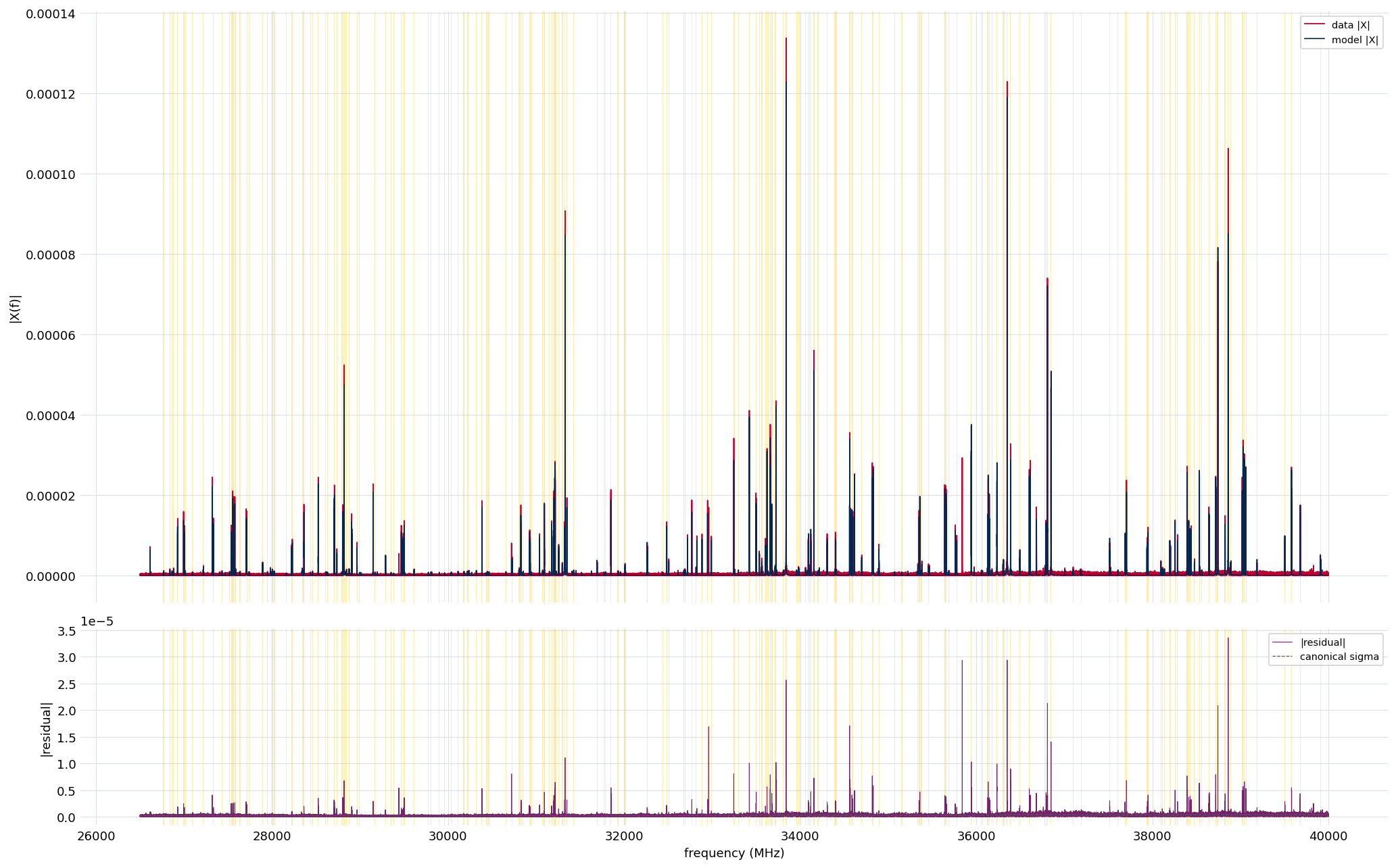
Stage 5 fit of the example experiment. Top: the fitted model (navy) overlaid on the active spectrum (red, magnitude), with the fit windows shaded gold. The model tracks the data across the full dynamic range — the strong lines and the weak forest alike. Bottom: the magnitude residual (purple) against the per-bin noise (gray dashed); across the band the residual sits at the noise level, the signature of a complete fit that has neither left real lines unmodeled nor manufactured spurious ones.

Choosing the shape and the calibration. The envelope shape is normally inherited from the Stage 2b line-shape vote, which also stamps the matching decay-time calibration. Pass --shape gaussian (or shape= on the Python interfaces) to fit the Gaussian envelope and consume the Gaussian \(\tau_G\) calibration instead; omit it to take the resolved default. A hand-tuned decay anchor can be supplied for an A/B test with --tau-maj-override / --sigma-tau-override (an atomic pair). Settings resolve in the usual order (explicit flags, then a persisted record, then a preset, then the recommended values, then the hard defaults) as described on Settings and presets. The packaged defaults preset is a copy-and-edit template of every knob at its default; a preset composes with explicit flags.

Inspecting, assessing, and tuning the fit

Three tools close the loop of looking at a fit, grading it, and adjusting it: fit show to inspect, fit check to grade, and the knobs to tune.

Inspecting. With no selector, fit show draws the spectrum-wide overview above (the model overlay and the magnitude residual), the view for confirming the residual sits at the noise level everywhere. Window selectors (--window, --window-list, --freq, --top-snr, --all-windows, --random) draw a consolidated per-window detail instead: the real, imaginary, and magnitude data with the model overlaid, the residual panels, a residual histogram, and a table of the fitted peaks with their uncertainties, alongside the printed fit log for that window. The detail figure is the tool for understanding why a window fit the way it did. By default the command opens an interactive window; --no-interactive with -o saves a static image.

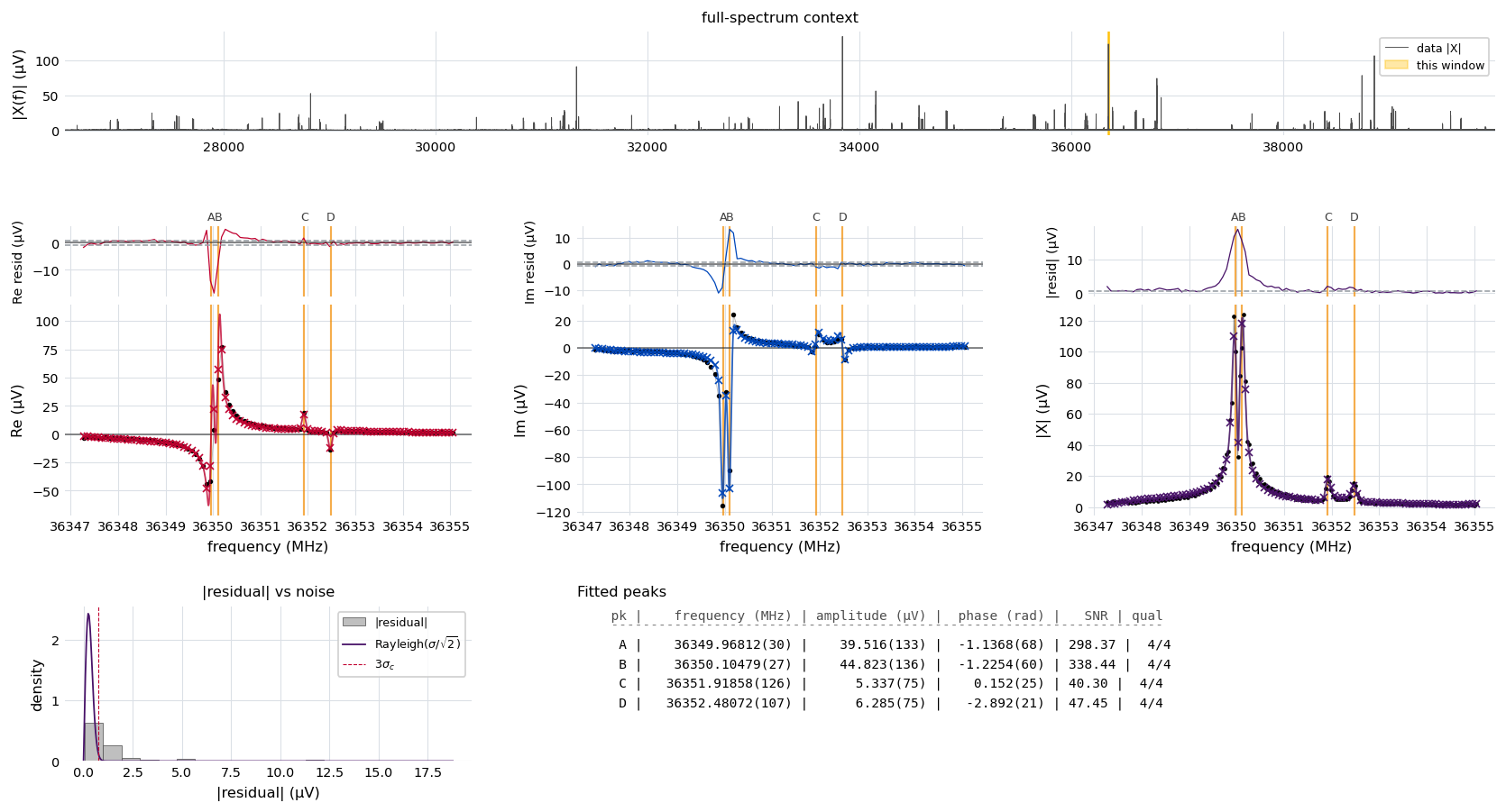
Per-window detail for a single window of the example experiment. The top strip locates the window in the full spectrum. The real, imaginary, and magnitude panels show the data (points) with the fitted model (lines, model values marked at the data bins) and the residual above each. The window holds two doublets — a strong, well-separated pair near \(36350\) MHz (signal-to-noise \(\approx 300\)) and a weak pair near \(36352\) MHz (signal-to-noise \(\approx 40\)). The residual histogram tracks the Rayleigh noise expectation, and the table lists each fitted line’s frequency, amplitude, phase, and signal-to-noise with the fit uncertainty on the trailing digits, plus a qual determinacy score (below). All four lines score 4/4: the fit determines each one, the weak doublet as firmly as the strong, so the score reflects how well the data pin a line rather than how bright it is. Determinacy is not strength.

The qual column is a per-line determinacy score — how many of four independent checks the line clearly passes, written k/4. The four checks are detected with margin (signal-to-noise comfortably above the survival floor), amplitude identifiable (the amplitude variance-inflation factor is well below the degenerate-collapse bar), position pinned (the frequency uncertainty is under a tenth of a resolution element), and isolated (no fitted neighbor within a resolution element). Each check reuses a threshold the pipeline already applies elsewhere, so the score introduces no new tuning. It measures how firmly the data determine a line, not whether the line is a real, assignable transition — a high score can still attach to an unmasked spur or an unassigned feature, which is why it informs curation rather than gating it.

Adding --rescue to any per-window selector emits a companion figure that traces how the residual-rescue pass built that window: the data and model, the final residual with each rescue round’s candidate nominations marked on it — filled where a nomination became a retained line, open where it was rejected or pruned — and a summary of the per-round \(\chi^2\) descent and peak budget. It renders from the persisted rescue record, so it needs no re-fit; it is the view for seeing which weak lines the rescue recovered and which it correctly declined.

Grading. fit check grades a completed fit against a signal-to-noise-aware acceptance framework: it flags windows whose reduced \(\chi^2\) exceeds what the local noise regime allows (a high-SNR window is held to a tighter standard than a faint one), reports the model-deficit tier, and, given a catalog of expected frequencies, runs a match check so unexplained residual structure stands out. It is read-only; it grades the fit without changing it.

Tuning. The defaults are calibrated for the reference instrument and generalize across a wide signal-to-noise range; routine use needs no adjustment. The most commonly touched knobs are below. Set them with per-knob flags on fit run, through a preset, or via settings=StageFitSettings(...) on the Python interfaces.

Knob	Default	Role
shape	lorentzian	Per-line envelope: lorentzian (\(e^{-t/\tau}\)) or gaussian (\(e^{-(t/\tau_G)^2}\)). Normally set by the Stage 2b vote.
tau.fit_tau_min_snr	10	In-window SNR above which the decay time is fit freely; below it, \(\tau\) is held at the Stage 2b majority value.
tau.per_band_tau	True	Anchor \(\tau\) to the per-band majority (True) or one band-wide value (False).
conservative.significance	0.05	Significance \(\alpha\) for the recorded F-test diagnostic and the rescue cleanup test. The main accept gate is the window-size-independent penalized bar (see the methods note), not this \(\alpha\).
rescue.snr_threshold	2.5	Residual-peak nomination floor for the rescue pass (nominates generously; the F-test gates acceptance).
thaw.residual_edge_threshold	8	Edge-coherence above which a window edge triggers the thaw / replan handshake.
baseline.edge_threshold	3.5	Edge-coherence above which the leakage-wing baseline is added to a window.
spur.enabled	True	Detect and mask clock/LO spurs (integer-megahertz CW tones).
peak_survival.snr_survival_factor	1.1	Sets the survival-cleanup floor as this multiple of the Stage 3 promotion cutoff. Set peak_survival.snr_survival_floor to pin an absolute floor instead.

The full knob set — the seeder thresholds, the per-window peak and separation caps, the phase/amplitude penalties, the rescue merge tiers, the spur and clock declaration knobs, and the survival/VIF parameters — is grouped into sub-settings (tau, seeder, conservative, penalties, rescue, thaw, spur, baseline, doublet_alternative, peak_survival) and reached through a preset or a settings bundle. Use scan to sweep a knob and see its effect rather than guessing.

Outputs and the handoff to Stage 6

A completed Stage 5 run stores a self-describing fit record: the per-window fit results and the merged, frequency-sorted global line list (each line tagged with its originating window); for every line the amplitude, frequency, phase, decay time, and their uncertainties from the fit covariance; the per-window audit trail (every candidate tested, its F-statistic, p-value, AIC, and the accept/reject decision); the thaw and replan histories; the rescue rounds; and the resolved parameters used, so the fit can be reproduced and reviewed. Like the earlier stages it is persisted in a flat, inspectable form rather than recomputed on demand.

For example, reloading the record exposes each line’s fitted parameters with their covariance uncertainties, its originating window, and its provenance:

fit = ftmw.load_fit("exp_2638.ftmw")     # the persisted fit record
pk = fit.fitted_peaks[0]                  # one line on the merged, frequency-sorted list
pk.frequency_mhz, pk.frequency_error      # frequency and its covariance uncertainty (MHz)
pk.amplitude, pk.phase                    # the other free per-line parameters
1.0 / pk.decay_rate                       # decay time tau (us); decay_rate is stored as 1/tau
pk.snr, pk.window_id, pk.origin           # SNR, originating window, "auto"/"user" provenance

The per-window detail figure above renders exactly this stored record for one window (the fitted parameters, the residual, and the add-loop decisions), so it is a concrete picture of what the fit persists.

Each rescue candidate the add never installed is also carried with its leftover signal-to-noise re-measured on the final residual, not the early-pass value that first nominated it, so the revival ledger Stage 6 builds from these candidates reflects the signal still genuinely unmodeled at convergence.

The fitted line list is the substrate for Stage 6, where it is reviewed, curated, and turned into the final products. Hand-edits (adding a line the fit missed, removing a spurious one, accepting or overruling a flagged merge) are made there through the review surface, which performs a single-window refit and marks the window as user-edited so the provenance of every line is preserved. A line a user adds (origin = "user") is immune to the automatic survival prune. Stage 6 reads the fitted line list, the per-window audit and renegotiation histories, the covariance-derived uncertainties, and the survival/attention flags to drive the review surface and the final reports.

Limitations

• The fit is prior-free: it claims a sub-resolution split only on the data’s own evidence, and where that evidence is ambiguous it merges and flags for review rather than guessing. Resolving a genuine close doublet against an over-split is a curation decision, supported by the observation-only doublet statistics and, where available, a catalog.

• The reported uncertainties are the formal fit (precision) uncertainties from the covariance. Systematic frequency accuracy, the absolute calibration of the instrument’s clocks, is a separate budget addressed by the clock declaration and the Stage 6 reports, not by the per-window fit.

• The line shape is the finite-acquisition damped cosine in the recommended envelope. A spectrum whose lines genuinely depart from both available shapes would show structured residual; fit check and fit show are the tools for spotting it.

With the lines fit and their parameters and uncertainties recovered, Stage 6 reviews the fit and produces the final line list and reports.