Complex-edge coherence statistic

The Stage 4 windowing stage cuts the spectrum into disjoint fit windows, and a boundary must fall where a strong line’s leakage has actually decayed into the noise — not merely where the magnitude spectrum looks flat. A finite acquisition spreads a bright line’s energy through truncation leakage whose skirt decays only as \(1/|\Delta f|\), several megahertz wide, and a boundary drawn through that skirt mis-attributes the line’s power to the neighboring window.

The leakage is invisible to a magnitude test. Its skirt is phase-coherent — it inherits the source line’s phase and rotates smoothly with frequency offset — so its magnitude passes through zero at every sinc null, and a fully coherent leakage tail can look exactly like noise in \(|X|\). The discriminator is phase: a coherent sum of complex bins grows like the number of bins over a leakage tail (the phases align), but only like the square root of the number of bins over noise (the phases are random).

Stage 4 therefore screens each band with a normalized coherent sum — the edge-coherence statistic — whose null distribution is known in closed form. This note derives that null, calibrates the operating threshold from the leakage amplitude the stage should act on, shows why the statistic must be scored in the active-region frame (and what de-ramping it a second time does), and validates it on the reference experiment. The figures and numbers are regenerated by docs/source/methods/edge_coherence/generate.py; see Reproducing this note.

Coherent sum and closed-form null

For an \(M\)-point band of complex spectrum values \(z_1,\dots,z_M\) with per-bin complex noise RMS \(\sigma\), the edge-coherence statistic is the modulus of the coherent sum, normalized so that pure noise gives an \(O(1)\) value independent of the band width:

\[S_\text{coh} = \frac{\bigl|\sum_{k=1}^{M} z_k\bigr|}{\sigma\,\sqrt{M}}.\]

Under the null hypothesis that the band carries only noise — independent complex Gaussian bins \(n_k\) with \(\mathbb{E}[|n_k|^2]=\sigma^2\) — the partial sum \(\sum_k n_k\) is itself complex Gaussian with variance \(M\sigma^2\). Its modulus is Rayleigh-distributed with scale \(\sigma\sqrt{M/2}\), so dividing by \(\sigma\sqrt{M}\) gives a statistic whose moments are

\[\mathbb{E}[S_\text{coh}\mid\text{null}] = \sqrt{\pi/4}\approx 0.886, \qquad \mathrm{Var}[S_\text{coh}\mid\text{null}] = 1-\pi/4\approx 0.215.\]

Both are independent of \(M\). That independence is the purpose of the \(\sqrt{M}\) normalization: it lets a single threshold serve every band width the stage might use. Sampling clean complex-Gaussian noise across band widths reproduces the closed form:

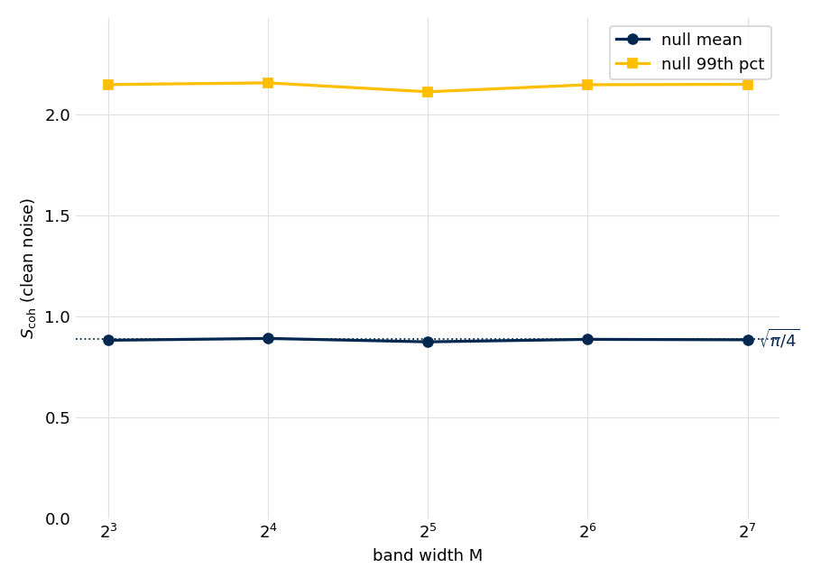
The null mean and 99th percentile of \(S_\text{coh}\) on clean noise, across band widths \(M=8\) to \(128\). The mean sits on \(\sqrt{\pi/4}\) and the 99th percentile on \(\approx 2.15\), both flat in \(M\).

Signal growth and the operating threshold

Under a coherent leakage tail of per-bin amplitude \(L\), the bins add nearly in phase, so \(|\sum_k z_k|\sim ML\) and the statistic grows as the square root of the band width against a contamination of fixed amplitude:

\[S_\text{coh} \sim \frac{ML}{\sigma\sqrt{M}} = \frac{L}{\sigma}\,\sqrt{M}.\]

The null stays put while this climbs, so doubling the band width buys \(\sqrt{2}\) more discriminating power.

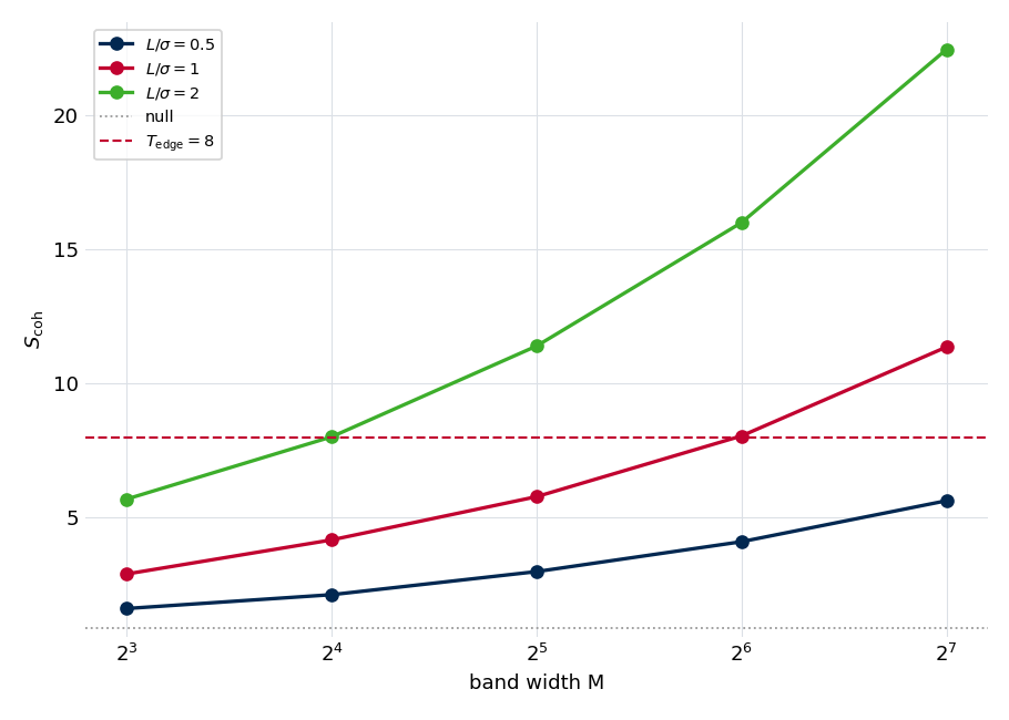
\(S_\text{coh}\) over a coherent band of per-bin amplitude \(L\), versus band width, for three \(L/\sigma\). The coherent value climbs as \(\sqrt{M}\) while the null (dotted) stays at \(\sqrt{\pi/4}\); a per-bin leakage of \(1\sigma\) reaches the operating threshold at \(M=64\).

The null only bounds the threshold from below. At \(S_\text{coh}=3\) the per-band false-positive rate is already well under a percent (the null 99th percentile is \(\approx 2.15\)), and a higher threshold makes it smaller still. What fixes the working threshold is instead how large a real leakage the stage should act on. Inverting the signal relation, the per-bin leakage flagged at a threshold \(T_\text{edge}\) over a band of width \(M\) is

\[\frac{L}{\sigma} = \frac{T_\text{edge}}{\sqrt{M}},\]

so the defaults \(T_\text{edge}=8\) and \(M=64\) flag coherent leakage of at least about one \(\sigma\) per bin — the \(L/\sigma=1\) curve in the figure crossing the threshold exactly at \(M=64\). A threshold near the null, say 3, would instead act on sub-\(\sigma\) leakage and read a large fraction of a line-dense spectrum as touched.

Scoring frame: the active-region transform

A coherent sum is only coherent in the right reference frame. A line that turns on at \(t_0=\) start_us inside the record carries a phase ramp \(e^{-i 2\pi f t_0}\) on every bin of a full-record transform; across a 64-bin band that ramp winds through several full turns, so a coherent sum over a full-record spectrum would cancel on genuine leakage and collapse the statistic to the null.

The statistic must therefore be referenced to the active-region turn-on, which the pipeline gets for free: it is scored on the canonical active FT — the transform of just the active region \([t_0,\,t_0+T]\) — which begins at the turn-on, so the spectrum is already in the line’s own \([0, T]\) frame and carries no ramp. The coherent sum is taken directly. The corollary is that the statistic must be evaluated in exactly one frame: scoring it on a full-record transform, or de-ramping the active FT a second time, reintroduces the ramp and collapses \(S_\text{coh}\) to the null.

Validation on the reference experiment

On the reference active FT the statistic separates the spectrum as intended. Strong lines tower over the threshold — the line near 36350 MHz reaches \(S_\text{coh}\approx 89\) with a contiguous above-threshold run several megahertz wide — while long stretches between clusters sit near the rolling-band null. Thresholding at \(T_\text{edge}=8\) marks about 6.6 % of the band as leakage-touched.

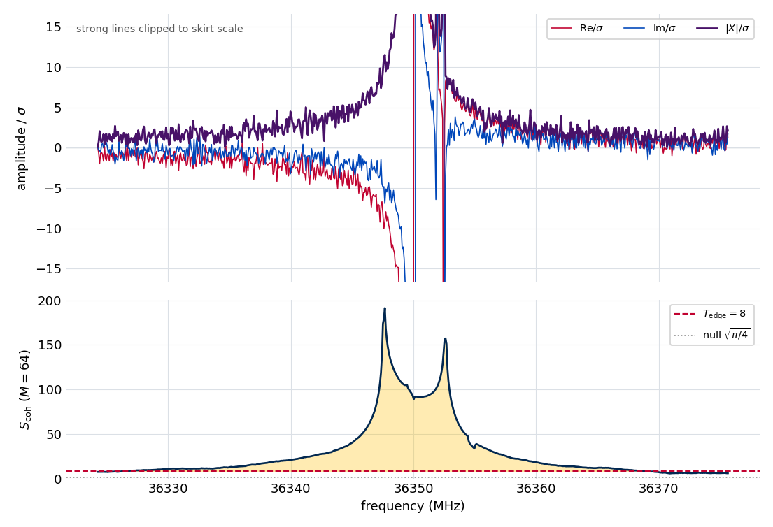
The 36350 MHz strong line on the reference active FT, in local-SNR units. The magnitude \(|X|/\sigma\) is clipped so the leakage skirt reads: away from the core the magnitude decays toward the noise, yet the real and imaginary parts keep oscillating coherently across it. The rolling \(S_\text{coh}\) (lower panel, \(M=64\)) towers far above the \(T_\text{edge}=8\) threshold across the whole leakage-touched span (gold fill), settling back toward the null \(\sqrt{\pi/4}\) only well away from the line.

The twin-peaked profile in the lower panel is a property of the statistic, not a pair of separate detections. In a line’s skirt the leakage is nearly pure dispersion — the quadrature lineshape, which is odd about the line center — so a band centered exactly on the line sums equal and opposite dispersive contributions that cancel, leaving only the smaller absorptive part. Shifted to either side the cancellation breaks and the net dispersive sum lifts \(S_\text{coh}\), so the statistic peaks just off the line and dips at its center; a synthetic isolated line reproduces the same symmetric pair. The blend here (a weaker companion near 36352.5 MHz) reinforces the right peak.

Two properties matter for trusting it there. First, the per-bin noise must be the local value: the Stage 2 noise varies by a factor of \(\approx 2.6\) across this spectrum, so a global median would understate significance in quiet stretches and overstate it in noisy ones. Second, there must be no pedestal: a constant complex offset would dominate the coherent sum linearly, but in a quiet region the median real and imaginary parts come in at \(-0.02\,\sigma\) and \(+0.08\,\sigma\) — consistent with zero, as a mean-subtracted FID requires.

Caveats

• One turn-on per record. The active-FT frame assumes a single active window; a multi-segment or re-triggered acquisition would carry more than one turn-on and is out of scope.

• The statistic locates, it does not identify. A reading above threshold says a coherent skirt reaches the band; which line it belongs to comes from the Stage 3 promoted-peak list. A threshold crossing with no nearby strong line is the signature of an undetected line — a diagnostic flag, not something to absorb silently.

• The map drives grouping, not attachment. The leakage-touched regions decide which strong lines are mutually coupled (the strong-cluster grouping); the fixed contributors a window carries are chosen separately, by the predicted skirt amplitude on that window’s grid (see Stage 4: Window Assignment).

• Interference can locally suppress the statistic. A coherent sum can be pulled down where leakage is still present: the dispersive cancellation at a line center, or destructive interference between two lines’ leakage in a blend, dips \(S_\text{coh}\) — in principle below threshold — and can split or shorten a leakage-touched run. The \(M\)-bin band smooths the statistic and a strong line’s central dip stays well above threshold (in the figure it falls only to \(S_\text{coh}\approx 90\)), so this bites only on finely-tuned cancellations, but a boundary drawn at such a dip would sit in still-contaminated spectrum.

Reproducing this note

The synthetic calibration and the 2638 application both call the shipped coherence_statistic() and active_edge_coherence(). Regenerate the figures and results.json from the repository root with:

python docs/source/methods/edge_coherence/generate.py

The synthetic null and signal-growth sweeps are a few seconds; the 2638 section builds the example experiment through noise estimation. Two fast, data-free invariants are exercised by the unit suite — the closed-form null mean and its \(M\)-independence, and the \(\sqrt{M}\) signal growth — and the 2638 numbers are guarded against drift by a slow-marked test.