Stage 2b: Decay-Time Calibration

Overview

A molecular free-induction decay rings down with a characteristic time constant \(\tau\). That decay time sets the natural linewidth of every peak (a longer \(\tau\) is a narrower line), so the per-window fit in Stage 5 needs a good starting value and a sensible prior for it. Stage 2b measures \(\tau\) directly from the raw FID, before any peak is detected, and produces a single data-driven decay time \(\tau_{maj}\) with a robust spread \(\sigma_\tau\), optionally broken down by frequency band. The same machinery also recommends which line shape the fit should use.

Stage 2b sits between Stage 2 (noise) and Stage 3 (peak detection). It is optional — Stages 3 and 5 run without it and fall back to a default decay time — but running it lets the fit anchor its line widths on the instrument’s real decay physics rather than a guess.

A completed run persists, for the chosen line shape:

• \(\tau_{maj}\) and \(\sigma_\tau\) — the band-wide majority decay time and its robust spread;

• per-band majorities — the same quantity computed separately on frequency bands (by default, the three arithmetic thirds of the analysis range), which the fit can route to window-by-window;

• a clock-spur catalog — the constant-magnitude (non-decaying) bins, grouped into one entry per tone, which later stages use to mask instrumental artifacts;

• a set of acceptance flags recording whether the calibration is well-determined;

• a line-shape recommendation stamped onto the file for Stages 3 and 5 to read.

Method

Stage 2b measures \(\tau\) in four steps, none of which runs a least-squares peak fit. It slides a short analysis window across the FID and, for each frequency bin, reads how the magnitude decays from one window position to the next — a single-parameter read of the decay rate, with no peak model and no blend ambiguity. Each bin is classified from that decay: a real molecular line decays, a clock spur holds constant, and noise or contaminated bins give no clean decay and are set aside. The surviving contributors’ decay rates are aggregated into a signal-to-noise-weighted majority \(\tau_{maj}\), optionally split by frequency band. Separately, the strong on-line bins are fit to three candidate line shapes and voted on to recommend which shape Stage 5 should use. Each step is expanded below.

Sliding-window STFT

For a single damped cosine \(s(t) = A\,e^{-t/\tau}\cos(2\pi f_0 t + \phi)\), take a short sub-interval of length \(T_w\) starting at time \(a\), zero everything outside it, and transform the full-length record. The on-line magnitude is

\[|S(a, f_0)| = \tfrac{1}{2} A\,\tau\,\bigl(1 - e^{-T_w/\tau}\bigr)\,e^{-a/\tau} = \text{constant} \times e^{-a/\tau}.\]

Sliding the window start \(a\) across the record traces out a pure exponential in \(a\) whose rate is \(1/\tau\) directly — a single-parameter read, with no least-squares peak model and no blend ambiguity.

The same construction applies to a Gaussian-decaying line. For \(s(t) = A\,e^{-(t/\tau_G)^2}\cos(2\pi f_0 t + \phi)\), a window short against the decay traces the Gaussian envelope instead of the exponential one,

\[|S(a, f_0)| \approx \text{constant} \times e^{-(a/\tau_G)^2},\]

so the per-bin series is read against a Gaussian in \(a\) with \(\tau_G\) as its single parameter. The two envelopes are alternative-shape models of the same underlying decay (one forces a pure-exponential ring-down, the other a pure-Gaussian one), not two decay times the molecule has at once. The line-shape recommendation below decides which variant the fit consumes.

The calibration splits the active region into n_seg non-overlapping windows (default ten), so each frequency bin yields a short time series of magnitudes versus window position.

The transform is taken at the full record length with the window’s samples in place and the rest zero-filled, never on the truncated window. Zero-filling preserves the full-record bin spacing \(\Delta f = 1/T_\text{full}\), so every frame shares one frequency grid and the per-bin time series are directly comparable. Truncating to \(T_w\) would double the bin width and break the comparison.

The behavior of each kind of bin across the frames is the basis of the method:

Bin	Magnitude versus window position
real molecular line	exponential decay \(e^{-a/\tau}\)
clock spur (continuous tone)	constant — no decay
noise bin	random walk, no clean exponential
skirt of a strong line	same decay rate as its parent line

Because a line’s leakage skirt decays at the parent’s rate, skirt bins reinforce the real-line cluster in the histogram rather than forming a spurious one.

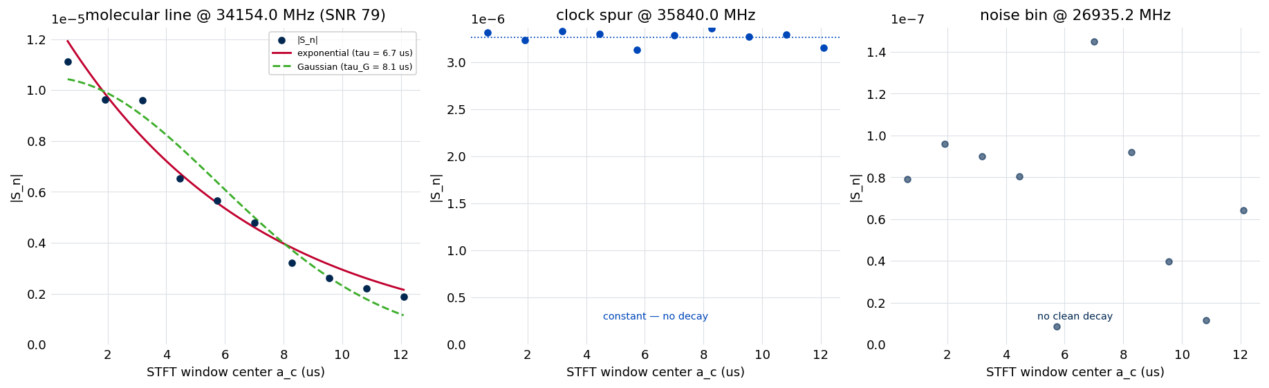
The per-bin magnitude-versus-window series the classifier fits, for three representative bins of the example experiment. Left: a strong molecular line, with the exponential and Gaussian decay fits overlaid — its decay time is the single parameter each contributor bin reports, and the two shape fits are what the line-shape vote compares. Center: a clock spur, constant across the windows. Right: a noise bin, with no clean decay. The three classes are visually distinct, which is what makes the fit-free read robust.

Classifying each bin

At each frequency bin the calibration fits the magnitude-versus-position series to the decay envelope being calibrated and sorts the bin into one of four classes:

1. Discard — the strongest frame’s magnitude is below t_sigma times the per-frame noise floor. Most bins land here.

2. Spur — a small-sample information criterion (AICc, defined under Line-shape recommendation) prefers a constant model over the decay, or the fitted decay time saturates against its upper bound (a continuous tone has effectively infinite \(\tau\)).

3. Bad fit — the fit residual is too large, marking dense or contaminated bins (overlapping skirts, mid-blend positions) that should not enter the histogram.

4. Contributor — everything else. These bins carry the decay times that are aggregated into \(\tau_{maj}\).

The per-frame noise floor comes from the FID tail, not the Stage 2 spectral \(\sigma\). The tail slightly over-estimates the true noise because it still carries decaying signal, and that inflation is deliberately kept: it acts as a stricter above-threshold gate that admits only well-determined on-line bins, which is what holds the per-band decay times on an independent fit-based reference.

The bad-fit gate is shape-matched: it tests the residual of the envelope the run is calibrating (the exponential for a Lorentzian run, the Gaussian \(e^{-(a/\tau_G)^2}\) for a Gaussian run), so a Gaussian-decaying line is not branded a bad fit by an exponential model that was never meant to describe it (the line-shape recommendation below, which fits all three candidate shapes, keeps a bin when the best of the three describes it well). A bin fails the gate when its residual sum of squares exceeds a hybrid threshold: the larger of a noise-scaled bound (a multiple rss_gate_factor of the per-frame noise) and a signal-scaled bound (a fraction relative_gate_fraction of the bin’s mean magnitude). The signal-scaled branch keeps clean, high-signal bins from being over-rejected, because the fast log-linear fit’s residual grows with the signal level rather than with the noise.

From contributors to a decay time

The contributor decay times are combined into a signal-to-noise-weighted majority: a weighted median, with each bin weighted by its on-line signal-to-noise. Weighting collapses the estimate onto the strong on-line bins; a plain median is biased high by near-threshold skirt bins whose noisy fits tend to run long. The spread \(\sigma_\tau\) is the weighted interquartile range rescaled to a standard deviation.

Two refinements run on top:

• Polish. The fast log-linear per-bin fit carries a small positive bias at intermediate record-length-to-\(\tau\) ratios. One Gauss-Newton refinement step per contributor removes it. The polish is applied only to contributors below a signal-to-noise cap (polish_snr_cap), because the bias concentrates at modest signal-to-noise and the same step over-corrects the strongest bins.

• Per-band majorities. The same weighted majority is computed on contributor subsets inside each frequency band. A band with too few contributors falls back to the band-wide value, so a sparse band never introduces a worse local anchor.

A one- versus two-component Gaussian-mixture test runs on the histogram and flags multimodality. On a single-species recording the decay time is expected to be unimodal; a genuinely bimodal histogram is surfaced as a flag for a human to audit rather than acted on automatically.

Line-shape recommendation

The recommendation determines which line shape the fit should use, from the data. On the strong on-line bins it fits three candidate decay envelopes: the exponential \(e^{-a/\tau}\) (Lorentzian), the Gaussian \(e^{-(a/\tau_G)^2}\), and a Voigt envelope \(e^{-a/\tau_L}\,e^{-(a/\tau_G)^2}\) carrying both a Lorentzian and a Gaussian decay. It scores each by its AICc, the small-sample-corrected Akaike information criterion, which measures goodness of fit while penalizing the Voigt model for its extra parameter. Each bin votes for its lowest-AICc model, and the votes are tallied signal-to-noise-weighted so the strong on-line bins that actually constrain the shape dominate. The recommendation is the pure shape (lorentzian or gaussian) that leads by at least a set margin of the weighted vote mass (pure_margin_threshold, default 0.10); when neither pulls ahead it is left unset.

The Voigt model is a foil, not an output. It is included so that a bin of mixed character is not forced to vote for a pure shape it does not match, but the recommendation itself is only ever lorentzian, gaussian, or unset: the Stage 5 fit supports the two pure shapes, and Voigt vote mass is tabulated for diagnostics only. The verdict is stamped on the file as a recommended_shape attribute that Stage 3 and Stage 5 read.

Each shape variant is stored separately: the Lorentzian (exponential) result at /stage2b_tau_calibration and the Gaussian (\(\tau_G\)) result at /stage2b_tau_G_calibration. The Gaussian variant keeps only the bins where the Gaussian describes the data better than the exponential (by a reduced-\(\chi^2\) margin) and applies a higher signal-to-noise floor, so its eligible contributor pool is smaller.

When the recommendation is unset — no pure shape clears the margin, or the Voigt foil leads — Stage 5’s shape resolver falls through to its configured default, Lorentzian, and consumes the Lorentzian calibration’s \(\tau_{maj}\) (the per-band value where routing is on). The decay time is only ever the \(T_\text{active}/3\) default when no calibration for the resolved shape is on the file at all — Stage 2b was not run, or only the other shape’s twin is present. Because a default tau run always produces the Lorentzian calibration, the common path uses the measured decay time, not the fallback.

Running a Lorentzian or Gaussian calibration runs the recommendation automatically (controlled by auto_recommend, on by default) and, when the vote names the other shape, also builds that shape’s calibration — so a single call leaves the file with whichever decay time the fit will actually consume. The vote can also be run on its own.

Running the stage

Stage 2b requires Stages 0–2. The default (Lorentzian) calibration:

$ ftmwpipeline tau run exp_2638.ftmw

The Gaussian variant, and the shape vote on its own:

$ ftmwpipeline tau run --gaussian exp_2638.ftmw
$ ftmwpipeline tau recommend exp_2638.ftmw

The same operations on the Python interfaces:

import ftmwpipeline.api as ftmw

tau = ftmw.calibrate_tau("exp_2638.ftmw")                     # Lorentzian
tau_g = ftmw.calibrate_tau("exp_2638.ftmw", shape="gaussian") # Gaussian
rec = ftmw.recommend_shape("exp_2638.ftmw")

# or, object-oriented
from ftmwpipeline import Pipeline
pipe = Pipeline.open("exp_2638.ftmw")
tau = pipe.calibrate_tau()
tau_g = pipe.calibrate_tau(shape="gaussian")

Re-running Stage 2b invalidates the downstream stages that depend on it.

The defaults are calibrated for the reference instrument and need no adjustment for routine use. The behavior is controlled by the knobs below, set with per-knob flags on tau run (e.g. --n-seg), through a preset, or via settings=TauCalibrationSettings(...) on the Python interfaces; how explicit, preset, persisted, and recommended values resolve is described on Settings and presets.

Knob	Default	Role
n_seg	10	Number of sliding windows. More windows sharpen each per-bin decay fit but lower the per-window signal-to-noise.
t_sigma	5	Above-threshold gate: a bin’s strongest frame must clear this multiple of the per-frame noise to be considered.
rss_gate_factor	5	Strength of the bad-fit gate that rejects dense or contaminated bins.
relative_gate_fraction	0.05	Signal-proportional branch of the bad-fit gate, needed so clean high-signal bins are not over-rejected.
min_contributors	200 / 50	Acceptance floor on the contributor count (Lorentzian / Gaussian).
sigma_tau_fraction_max	0.20	Acceptance ceiling on the relative spread \(\sigma_\tau/\tau_{maj}\).
polish / polish_snr_cap	true / 9	Apply the Gauss-Newton bias-removal step, to contributors below this signal-to-noise.
compute_band_majorities	true	Compute the per-band decay times the fit routes on.
spur_cluster_multiplier	1.0	Adjacency, in analysis-grid bins, for collapsing neighboring spur bins into one tone.

The Gaussian variant adds its own knobs (the signal-to-noise floor snr_min, the \(\tau_G\) fit bounds, and the reduced-\(\chi^2\) eligibility margin delta_chi2r_min); the per-band split is configurable through band_edges_mhz and band_labels.

Inspecting the diagnostics

tau show renders two views (--gaussian selects the Gaussian group). The heatmap (--kind heatmap) shows the magnitude across the sliding windows and the analysis band, so real lines appear as streaks that fade down the window axis while clock spurs hold constant brightness:

$ ftmwpipeline tau show --kind heatmap exp_2638.ftmw

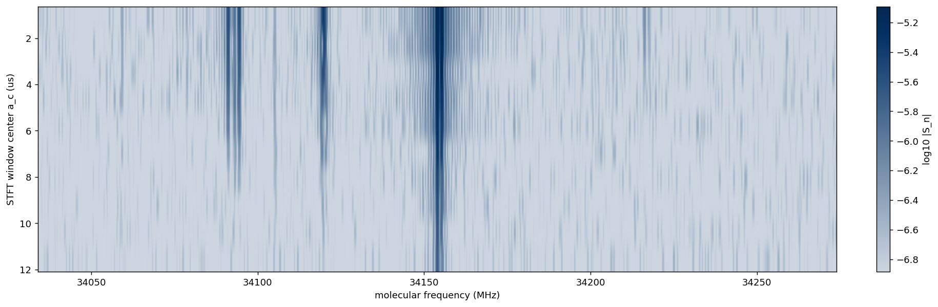
The STFT magnitude heatmap, zoomed to a strong-line neighborhood of the example experiment and with the color range clipped so the decays read. Window position runs from the earliest at the top to the latest at the bottom; a real line is a column that is darkest at the top and fades downward, while a clock spur holds the same shade down the whole column.

The distribution view (--kind distribution) shows the contributor histogram and the recovered decay time:

$ ftmwpipeline tau show --kind distribution exp_2638.ftmw

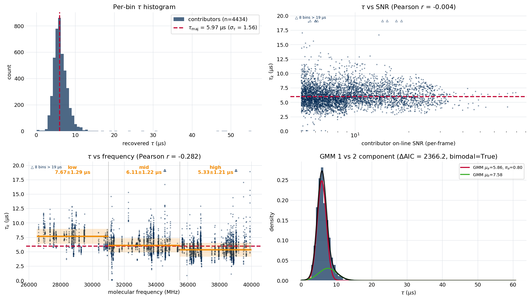
The decay-time distribution on the example experiment. Top left: the contributor histogram with the signal-to-noise-weighted majority \(\tau_{maj}\) overlaid. Top right: per-bin decay time versus signal-to-noise. Bottom left: decay time versus molecular frequency, with each per-band majority drawn as a level and its robust spread \(\sigma_\tau\) shaded — the band-to-band trend the per-band routing captures. Bottom right: the one- versus two-component Gaussian-mixture fit used for the multimodality flag. The two decay-time scatters cap their axis at one and a half times the active-region length, because decay times beyond that are not reliably measurable, and flag any contributor above the cap as an open triangle along the top edge.

The same figures are available from Python through ftmwpipeline.api.visualize_tau_distribution() and ftmwpipeline.api.visualize_tau_heatmap() (and the matching Pipeline methods), each taking a shape argument.

When to trust the calibration

The calibration always returns a decay time, but it records whether that value is well-determined through three acceptance pre-conditions: enough contributors, a relative spread \(\sigma_\tau/\tau_{maj}\) below sigma_tau_fraction_max, and no strong unexplained bimodality. Failing a pre-condition logs a warning and sets preconditions_passed to False but does not block the downstream stages from consuming \(\tau_{maj}\) — the flag is guidance for the analyst, not a gate. On a band whose decay time genuinely varies with frequency, the band-wide spread can exceed the ceiling while each per-band spread stays comfortably inside it; the per-band majorities are then the values to trust.

Frequency dependence

On the reference instrument the decay time decreases smoothly from the low end of the band to the high end — roughly a third shorter across the W-band span. This is a real, reproducible structure, not scatter: the per-band sampling error is far smaller than the trend. It is consistent with the transmit/receive horn geometry (a fixed-gain horn’s beamwidth narrows with frequency, so the molecular beam spends less time in the coherent interaction region at higher frequency, shortening the observed decay). Because the trend is geometric rather than molecular, the per-band decay times (not a single global value) are the faithful description, which is why per-band routing is on by default.

What the later stages consume

• Stage 3 reads the recommended shape and the matching decay time as the basis for its gap-pass matched filter.

• Stage 5 uses \(\tau_{maj}\) (or the per-band value for each window, when per-band routing is on) as the starting decay time and as the center of a bidirectional prior that resists both over-broadening and over-narrowing of the fitted lines, and consumes the spur catalog to mask instrumental tones. The \(\sigma_\tau\) that sets the prior width is floored so a very tight histogram cannot make the prior over-confident.

Limitations

• The strongest on-line bins are classified as bad fits, because real lines are not pure single exponentials; their decay times are excluded. The contributor population is nonetheless large and representative.

• A spur whose leakage skirt overlaps a real line within about one analysis-grid bin can capture that line into the spur class. Lines that close to a strong tone were unlikely to fit cleanly in any case.

• Genuinely multi-species recordings, where a minor histogram cluster is a distinct species rather than a band-of-the-same-species effect, would need a per-species decay time; the calibration flags the multimodality but reports the dominant cluster.

The decay-time calibration is the last preparation step before Stage 3 detects peaks on the noise-referenced spectrum.