Scope-Record Import

Some instruments do not hand back a single averaged free-induction decay. A direct-sampling oscilloscope captures one long record — a quiet pre-record, a run of chirp/FID frames at a fixed repetition period, and a dead tail — and leaves the averaging and segmentation to the analyst. The segmentation is operator knowledge: nothing in the file says where the frames begin. Scope-record import brings such a capture into the pipeline, performs the record-changing transforms (frame averaging, ADC-offset cleanup) inside the pipeline so they land in the provenance, and keeps the diagnostic segments the later stages need.

The governing rule is that any transform that changes the science record happens in-pipeline. A scope record can always be averaged into a bare FID offline and imported through the generic csv or ftmw-hdf5 path, but then the provenance and the diagnostic segments are lost. Importing the raw record keeps both.

The segmented record

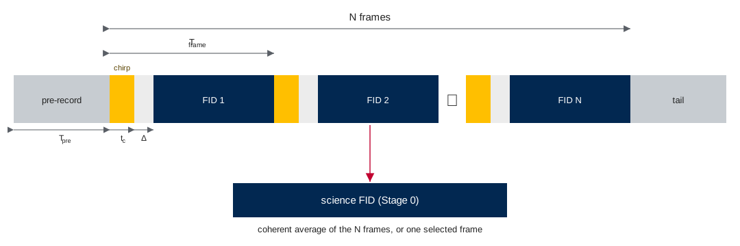
Schematic of a segmented scope record. — A segmented scope record (schematic, not to scale). One long capture holds a quiet **pre-record**, \(N\) **chirp/FID frames** at a fixed period, and a dead **tail**; each frame is a chirp excitation, a hold-off while the chamber settles, then the molecular FID. The science FID handed to Stage 0 is the coherent average of the frames, or a single selected frame. The pre-record — a stretch with no chirp excitation — is kept as a diagnostic segment because it anchors the chirp-response spur test. Symbols: \(T_\text{pre}\) pre-record duration; \(T_\text{frame}\) frame period; \(N\) frame count; \(t_c\) chirp duration; \(\Delta\) start hold-off (ring-down settling plus margin) after the chirp.

The import is parameterized by what the operator knows about the capture:

pre_record_us — the duration of the quiet segment before the first chirp;
frame_period_us — the repetition period of the frames;
n_frames — how many frames the record holds.

From those three the record is sliced into the pre-record, the per-frame array, and the tail. By default the frames are coherently averaged into the science FID (the averaging gain that a hardware-averaging instrument would have applied itself). Two options change that:

frame=k imports a single frame k as the science FID instead of the average — one .ftmw per frame, for per-frame or time-dependent analysis (it batches the same way Blackchirp writes one record per frame);
keep_frames retains the full per-frame array in the file (off by default; the frames are large and are discarded after averaging unless asked for).

The averaging is a plain mean — no robust averaging or frame rejection.

The shipped loader: keysight-mat

The layout parameters, averaging, interleave cleanup, chirp window, and pre-record anchor are all generic to the segmented-scope-record model; a per-vendor loader supplies only the raw samples and the acquisition metadata. One such loader ships today, keysight-mat, for Keysight oscilloscope .mat files (MATLAB v7.3, which is HDF5 underneath). It reads the raw samples and the sample clock, vertical scaling, and instrument identity, and is auto-detected from the .mat extension and the file’s channel structure. Other vendors’ raw formats are future sibling loaders feeding the same generic surface, not options on this one.

$ ftmwpipeline data import exp.ftmw scope.mat --format keysight-mat \
    --pre-record-us 12.5 --frame-period-us 20 --n-frames 19 \
    --interleave-factors 16,512

# Import one frame as the science FID instead of the average:
$ ftmwpipeline data import exp_f3.ftmw scope.mat --format keysight-mat \
    --pre-record-us 12.5 --frame-period-us 20 --n-frames 19 --frame 3

The same parameters flow through the functional API and the Pipeline constructor:

import ftmwpipeline.api as ftmw

ftmw.import_data(
    "exp.ftmw",
    source="scope.mat",
    format_name="keysight-mat",
    pre_record_us=12.5,
    frame_period_us=20.0,
    n_frames=19,
    interleave_factors=[16, 512],
)

A multi-channel file needs an explicit --channel (it defaults to the sole channel when only one is present). After import, data show prints the acquisition-segment map — the pre-record and tail lengths, the frame period and count, and whether the per-frame data was retained — alongside the usual FID summary.

Direct-sampling instruments digitize the molecular band directly (no down-conversion), so the probe frequency is zero and the digitized baseband is the molecular frequency. The rest of the pipeline treats the result like any other Stage 0 FID; the only difference is what import recorded along the way.

What import persists

Alongside the science FID, Stage 0 stores the acquisition segments — the pre-record, the tail, the segment map, and (only under keep_frames) the frames — plus the ADC-cleanup patterns if cleanup ran. The source provenance records the layout parameters, the frame selection, and the cleanup factors, so a re-import of the same source with the same parameters is a safe no-op, while a different frame selection or layout is recognized as a different import and re-runs the affected stages (see Stage 0 for the re-import contract).

The pre-record as a spur anchor

Keeping the pre-record pays off in Stage 5. A molecular line only exists if a chirp excited it, so a real line is absent from the pre-record (or weak, decaying from the previous frame’s chirp). An external interfering tone — a clock or LO leakage — is present in the pre-record at full strength because it does not need the chirp. Comparing the band power at a candidate frequency in the pre-record against the FID window is therefore a direct test of whether a “line” is instrumental:

ratio near one → present without the chirp → gate it as interference;
ratio near zero → only appears with the chirp → protect it as molecular;
in between → inconclusive, and the other spur lanes (the clock lattice, the decay probe) decide.

This chirp-response test runs ahead of the decay probe, because a modulated carrier can mimic an FID decay and fool a decay test — but it cannot hide from the pre-record. It only arbitrates tones bright enough to rise above the pre-record’s own noise floor (which is worse than the averaged FID’s by roughly the square root of the frame count); weaker candidates fall to the other lanes.

Interleave-offset cleanup

A high-rate digitizer is built from several slower ADCs interleaved in turn. Tiny fixed voltage offsets between those sub-converters repeat every M samples and appear in the spectrum as a comb of tones at multiples of f_s / M. Because the offsets are a fixed per-phase DC pattern, they can be estimated and removed.

The cleanup is opt-in and operator-declared. Passing --interleave-factors (for example 16,512) declares the interleave depths and runs the cleanup; omitting it suppresses the cleanup entirely. The depths are a property of the digitizer the operator supplies — they are not auto-detected from the record. When declared, the import estimates each per-phase mean on the raw pre-record samples (before voltage scaling, where the pattern is cleanest) and subtracts the tiled pattern from the whole record before slicing.

The cleanup is partial by design — part of the comb rides the signal path, not just the ADC, so the subtraction reduces but does not erase it. What it leaves behind is handled by the clock-lattice gate: the cleanup’s own f_s / M comb frequencies are written to the recommended clock declaration (as locked sources), so the spur lattice knows to expect them.

One subtlety matters for trusting the spur lane. The cleanup estimates its pattern on the pre-record, so it nulls those comb frequencies in the stored pre-record exactly. An unguarded chirp-response test would read that absence as “absent without the chirp” and wrongly protect a clock tone. The probe therefore returns inconclusive at the cleanup-comb frequencies and lets the lattice and decay lanes decide. The principle is general: any preprocessing estimated on a reference segment removes its own correction frequencies from that segment, so any later statistic on the segment must exclude them.

The chirp window and the FID start

The FID must start only after the excitation chirp and the switch ring-down have cleared. How long that takes is a property of the instrument — how quickly its chamber and switches settle — not of the digitizer; some instruments settle in a fraction of a microsecond, others ring for several (the example Keysight record is one of the latter, its chamber being lightly absorbed). Scope-record import declares the chirp window at import time (--chirp-start-us / --chirp-end-us / --start-margin-us), and the margin absorbs whatever ring-down the instrument has.

This feeds the same declared-chirp-window path Stage 0 start-time detection already uses: a declared chirp end sets the recommended start to chirp_end + margin and is treated as authoritative, with the energy-sweep detector running only as a cross-check that warns on disagreement. See the Stage 0 page for the detection mechanics; here the point is simply that the declaration travels in from the import. (A Blackchirp import derives the same window from the experiment configuration automatically.)

Interfaces

Scope-record import is the same Stage 0 import surface used everywhere, with the layout parameters added:

CLI — data import <file> <source> --format keysight-mat with --pre-record-us / --frame-period-us / --n-frames (required) plus the optional --frame / --keep-frames / --channel / --interleave-factors / --chirp-start-us / --chirp-end-us / --start-margin-us; data show surfaces the segment map.
Functional API and Pipeline — import_data(...) / Pipeline.create(...) take the same parameters as keyword arguments.

The segments and cleanup patterns travel with the .ftmw file, so a recipient reproduces the fit — including the spur decisions that depend on the pre-record — from the file alone.