Stage 5 fitting: gates, blends, and SNR-aware acceptance

Stage 5 (Stage 5: Peak Fitting) turns each window’s detected peaks into a fitted model by growing the model one line at a time, accepting a new line only when the evidence warrants it, with no molecular-physics prior to lean on. Two properties make that decision hard to get right. The accept test must be immune to window size, or the windowing choices of Stage 4 would silently change which lines survive; and the usual measure of a good fit, a reduced \(\chi^2\) near one, breaks down at the high signal-to-noise where the analytic line shape sits hundreds of standard deviations from a real line.

This note derives the acceptance gate that meets the first requirement and the health criterion that meets the second, shows how one gate handles the two discovery problems a prior-free fitter faces — blended lines and under-complete candidate lists — and validates the whole stage across roughly three decades of signal-to-noise on the seven checked-in experiments. The figures and numbers are regenerated from the shipped fitting code by docs/source/methods/stage5_fitting/generate.py; see Reproducing this note.

A window-size-invariant acceptance gate

Every add-one-line step asks the same question: do the data support another line, or is the apparent improvement just the extra freedom of a larger model fitting noise? Too lenient and the fit sprouts spurious lines on every strong line’s skirt and every noise excursion; too strict and it misses the weak lines detection worked to find. The test must also return the same verdict in a tight two-bin feature and in a wide window padded with hundreds of quiet bins — otherwise Stage 4’s window boundaries would change which lines survive.

The classical choice is the nested-model F-test: the more-complex model adds parameters and lowers the chi-squared, and the F-statistic

\[F = \frac{\Delta\chi^2 / \Delta k}{\chi^2_{K+1} / (n_\text{data} - k_{K+1})}\]

gates the addition through its p-value. It carries a structural bias that makes it the wrong tool here. The numerator is the local evidence for the candidate — the chi-squared drop \(\Delta\chi^2\), which lives in the handful of bins the new line informs. The denominator is the more-complex model’s reduced chi-squared over the whole window, which a converged fit drives toward one as the window fills with quiet bins at the noise, while the F-distribution’s second degree of freedom grows with the same bin count. Both effects push one way: for a fixed amount of local evidence, padding the window with quiet noise lowers the p-value. Significance is manufactured from empty bins.

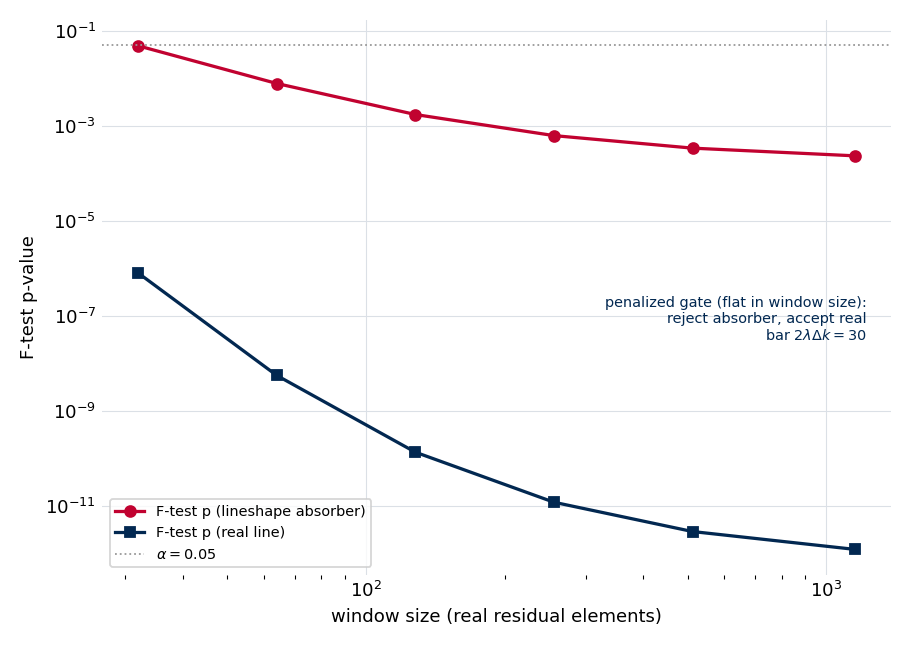
F-test p-value against window size for two candidates of fixed local evidence, padded with progressively more quiet bins. A marginal candidate absorbing a bright line’s irreducible lineshape misfit (red) starts at \(\alpha = 0.05\) in a tight window and is driven to high significance purely by padding — the F-test would accept it on a wide window. The shipped penalized gate compares the same local \(\Delta\chi^2\) to a fixed bar and returns the same verdict (reject the absorber, accept the real line) at every window size.

The figure makes the failure concrete: a candidate carrying a fixed \(\Delta\chi^2 = 20\) — a line really just absorbing the lineshape floor under a bright neighbor — has an F-test p-value of about \(0.048\) in the tightest window and about \(2\times10^{-4}\) once the window is padded to a thousand bins. Same line, same evidence; the verdict flips with the window geometry.

The fix is to gate on the quantity that does not depend on window size. Because the \(K\)-line and \((K{+}1)\)-line models compared at a step share the same window bins, the chi-squared difference \(\Delta\chi^2\) is purely the local likelihood-ratio statistic of the added line — the quiet bins contribute equally to both models and cancel. Stage 5 accepts the more-complex model when

\[\Delta\chi^2 \;>\; 2\,\lambda\,\Delta k,\]

a penalized-chi-squared bar with a single global strictness \(\lambda\). At \(\lambda = 1\) this is the textbook AIC rule (\(\Delta\chi^2 > 2\,\Delta k\)); the shipped \(\lambda = 5\) is a stricter, BIC-like bar. The reference experiment carries no ground-truth line list, so \(\lambda\) is not tuned to a target count; it is set so the gate’s borderline calls fall where a spectroscopist’s judgment is also uncertain, while plainly real and plainly spurious lines land decisively on either side. One added line costs \(\Delta k = 3\) parameters (amplitude, offset, phase; the decay time is shared at window level), so the bar is \(\Delta\chi^2 > 30\). It has no \(n_\text{data}\), no \(n_\text{eff}\), and no window geometry in it at all — the property the F-test lacked.

The gate replaced an intermediate form the audit trail still carries. The first fix for the F-test bias kept the AIC framework but shrank its sample size: an information-weighted effective sample size \(n_\text{eff}\) weighting each bin by \(\log(1 + \text{SNR})\), fed into the small-sample-corrected AICc. That removed the dilution but left the bar drifting with the weight distribution; scoring the window-size-independent \(\Delta\chi^2\) directly is the cleaner statement of the same idea. The classical F-statistic and its p-value are still computed and recorded at every step as a familiar diagnostic, but they no longer gate the decision.

Localizing the gate against the lineshape floor

A bare \(\Delta\chi^2\) bar has one remaining blind spot. At high signal-to-noise the finite-acquisition line shape is never a perfect fit to a real line — a sub-percent core residual is irreducible — and that misfit is reducible-looking: a spurious extra component placed on a bright line’s core can soak up the residual and earn a large \(\Delta\chi^2\), clearing the bar for the wrong reason. The discriminator is location. Residual sitting under a bright model component is the irreducible lineshape floor; residual sitting where the model is small is a genuine missing line. Stage 5 scores the gate’s chi-squared against a fidelity-inflated per-bin noise

\[\sigma_\text{eff}^2(f) = \sigma^2(f) + \bigl(\kappa\,|\text{model}(f)|\bigr)^2,\]

with \(\kappa\) the tolerated fractional model deficit. Where the model is bright, \(\kappa\,|\text{model}|\) dominates and the residual’s evidence is shrunk to the fidelity budget; where the model is small, \(\sigma_\text{eff} \to \sigma\) and the evidence keeps full weight. A frozen-skirt budget covers bright structure subtracted from the data and invisible to \(|\text{model}|\).

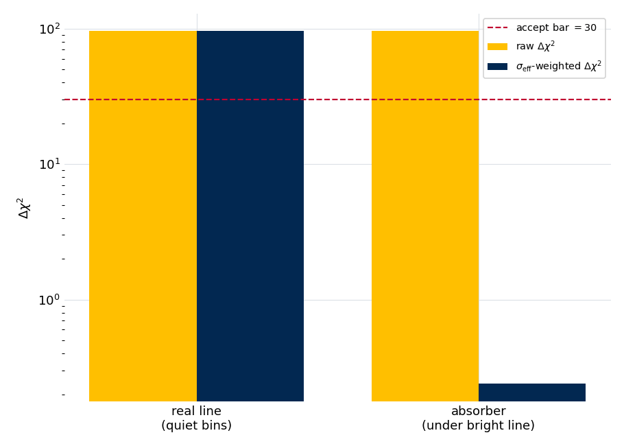
The same candidate evidence, scored two ways. Both candidates carry an identical raw \(\Delta\chi^2\) well above the accept bar (gold). Under the \(\sigma_\text{eff}\) weighting (blue), a real line over quiet bins keeps its full evidence and is accepted, while a candidate absorbing the lineshape floor under a bright line (on-line SNR 400) is discounted to a fraction of the bar and rejected.

In the synthetic test both candidates start at raw \(\Delta\chi^2 = 96\). Over quiet bins the \(\sigma_\text{eff}\) evidence is unchanged at \(96\), comfortably above the bar of \(30\); under the bright line’s core it collapses to \(0.24\), three orders of magnitude below the bar. The gate keeps the real line and rejects the absorber on the same nominal evidence, by reading where the residual sits.

One gate at every site

This penalized, localized gate is a single function applied at all four places Stage 5 weighs adding or removing a line: the conservative add-one-line accept test, the blend-aware seeder’s \(K{=}2\)/\(K{=}3\) escalation, the per-line knockout test, and the merge of close pairs. Using one criterion everywhere is what makes the fit’s behavior coherent — a line the accept gate admits is one the knockout gate will not immediately remove, because they ask the same question with the same bar.

Blends: detectable, but easy to mis-initialize

The hardest discovery a prior-free fitter faces is a blend: two lines closer than a linewidth. Fitting the unwindowed spectrum (the reason the canonical FT is left unapodized) is what makes it possible at all, but it raises two questions with very different answers — can a close blend be recovered, and will the sequential loop find it.

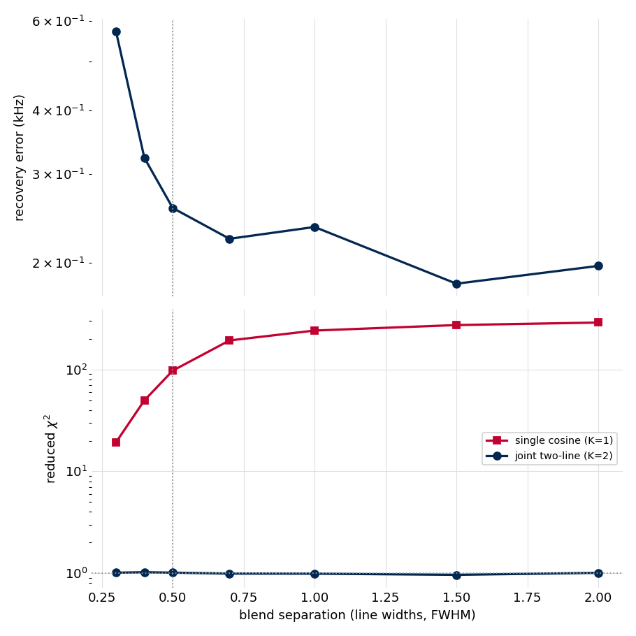
A 1:1 in-phase blend swept over separation, in line widths. Top: the frequency error of a joint two-line fit started at the true positions — recovery holds at the sub-kHz level down to 0.3 of a linewidth. Bottom: the reduced chi-squared of a single-cosine fit to the same blend (red) is elevated by one to two orders of magnitude across the whole range, while the joint two-line fit (blue) sits at one — so a blend always leaves an unmistakable single-line signature.

Recovery is excellent: given the right number of lines, a joint fit recovers a 1:1 blend at on-line SNR 120 to better than \(0.6\) kHz even at 0.3 of a linewidth, and to \(0.2\)–\(0.3\) kHz from half a linewidth outward — far below the nominal resolution. Detectability is never the limit either: a single damped cosine has one fixed shape, and a blend it cannot match leaves a reduced chi-squared of \(19\) at 0.3 FWHM rising to nearly \(290\) at 2 FWHM, against \(1\) for the correct two-line fit. The elevation is large, smooth, and present at every separation.

The limit is initialization. The conservative loop fits one cosine, lets it drift to the blend centroid, then tries to add a second from that drifted state — and for a tight, near-equal, in-phase blend that sequential path lands in a basin where the two cosines collapse together. The blend was always recoverable (top panel) and always detectable (bottom panel); the loop simply did not start the two-line fit well enough. This is why Stage 5 carries a blend-aware seeder: when a single-cosine fit leaves an elevated reduced chi-squared, it retries with two (then up to three) lines straddling the feature rather than stacked at the centroid. That escalation, not a large patience budget, is what resolves real doublets; the per-window line count is otherwise unbounded, and a width bound, not a count, holds the forest.

Residual rescue

The detector runs on the magnitude spectrum and trusts its candidate list. When that list is under-complete — a hyperfine multiplet whose strongest member masked the others, a line on a strong neighbor’s shoulder — the conservative loop converges to a model that absorbs the missing lines, leaving an above-noise, phase-coherent residual. The rescue is a second pass that re-examines that residual, and its structure is what keeps it well posed. Each round computes the residual against a properly joint refit of every line accepted so far, never a recursion on a shrinking residual against an ever-more-wrong model: recursing on the residual of the initial fit would propagate that fit’s errors (its wrong decay, its wrong amplitudes) forward as structure the rescue then chases. The rescue nominates generously from residual prominence, folds the candidates into the joint fit, gates each through the same penalized gate the main loop uses, and drops any line the refit no longer supports. It seeds from the converged decay time, except when the initial fit pinned the decay at its bound — the signature of a broken fit absorbing unmodeled residual — in which case it falls back to the calibrated Stage 2b value.

A leakage-wing baseline, a low-order complex polynomial added only on an F-test or edge-coherence trigger, carries the smooth pedestal that hundreds of distant lines’ summed leakage leaves under a window and that the discrete contributor set cannot model.

A sub-resolution pair the fit split into two lines is then adjudicated by the amplitude variance-inflation factor \(\text{VIF} = (\sigma_A/A)\cdot\text{SNR}\), the diagnostic that separates a resolved doublet from a least-squares over-split. When two components sit within a resolution element their amplitudes trade against one another: the covariance inflates and a member’s VIF climbs. A genuinely resolved doublet keeps its amplitudes individually constrained — across the catalog-checked fixtures its VIF stays moderate (\(\lesssim 20\)) — while an unidentifiable pair drives a member’s VIF far higher, so a threshold (default \(25\)) collapses only the unambiguously degenerate pairs to a single centroid line carrying a spread-inflated frequency uncertainty, and leaves the borderline ones split but flagged for review.

The bias toward merging is deliberate and asymmetric. In the ambiguous sub-resolution band a prior-free least-squares split is far more often a canceling near-duplicate artifact than a real doublet, and the two errors are not equal: merging a genuinely resolved doublet destroys a real line and cannot be recovered downstream, whereas a flagged over-split is recovered by review. The threshold therefore sits well above the resolved-doublet VIF range so only unidentifiable structure collapses, guarded by a footprint test that forbids a merge from folding across a real gap into a neighbor, and iterated to a fixed point. This does not contradict the sub-linewidth recovery above: the fitter can resolve a pair to 0.3 of a linewidth when told there are two lines (the blend study), while this criterion governs whether the pipeline keeps a sub-resolution split with no prior — a curation decision it surfaces rather than forces.

An SNR-aware health criterion

Judging a converged fit by a reduced chi-squared near one fails at high signal-to-noise, and fails where it matters: it would condemn the best fits in the spectrum. At on-line SNR of \(10^4\)–\(10^5\) the per-bin noise is so small that the irreducible sub-percent lineshape misfit is hundreds of standard deviations per bin, so a perfectly good fit of a bright line has a reduced chi-squared in the thousands. The honest health metric has two regimes,

\[\chi^2_r \;\le\; F + (\kappa\cdot\text{SNR}_\text{max})^2,\]

the SNR-aware acceptance gate. At low SNR the deficit term vanishes and the gate is the noise-regime allowance \(\chi^2_r \le F\) (with \(F = 3\) budgeting for the sampling scatter of a good fit); at high SNR the \((\kappa\cdot\text{SNR})^2\) term governs and a bright line that fits to its lineshape floor passes. The honest, SNR-independent measure of fit quality is then the fractional core residual

\[\varepsilon = \frac{\sqrt{\max(\chi^2_r - F,\, 0)}}{\text{SNR}_\text{max}},\]

how far the analytic shape departs from the real line. The \(\kappa\) here is the same fidelity budget that localizes the accept gate above: the window-level allowance and the per-bin \(\sigma_\text{eff}\) are two views of one number.

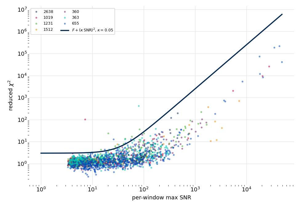
Per-window reduced chi-squared against per-window max SNR for every window of the seven checked-in experiments, each fit in its recommended line shape. The cloud follows the \(F + (\kappa\cdot\text{SNR})^2\) gate (blue), flat at the noise floor where lines are faint and rising as the lineshape floor at the bright cores. The same cloud looks “bad” under a flat \(\chi^2_r \approx 1\) standard and healthy under the SNR-aware one.

Cross-fixture validation

The defaults are tuned on one experiment (the gaussian-shaped reference at SNR up to a few hundred), so the question is whether they generalize. The seven checked-in fixtures span vinyl cyanide at SNR above \(30{,}000\), three methyl-rotor spectra, and several sparse ones — built fresh through Stage 5, each in the line shape its Stage 2b vote recommends, with no hand-tuning. Across all seven the SNR-aware gate clears at least 95 % of every fixture’s windows (pass rate \(0.95\)–\(1.00\)), and the per-window reduced chi-squared median stays between \(1.1\) and \(1.6\), from the sparse low-SNR spectra up to vinyl cyanide. The defaults calibrated on one experiment hold across the whole set without adjustment.

The two vinyl-cyanide fixtures carry a ground-truth catalog, which is what lets the cross-fixture set probe the two failure modes a line count cannot: overfitting (a fitted line with no catalog counterpart) and blend discrimination (whether a cataloged close pair is resolved or merged correctly). The catalog also bounds completeness directly: the fit recovers \(34\) % of the catalog’s in-band lines on the sparse fixture and \(52\) % on the dense, extreme-SNR one — a recall bounded by detectability, not fit quality, since the catalog includes lines below the spectrum’s noise that no fit can recover. Where a line is detected, its frequency is recovered to the instrument’s accuracy floor, and that floor — a few kilohertz of clock drift — is a property of the instrument, not the pipeline; the formal fit precision is far tighter, and the gap between them is the subject of the clock declaration and the Stage 6 reports.

Caveats

• The gate is calibrated, not derived from first principles. The reference experiment has no ground-truth line list, so the strictness \(\lambda = 5\) and the fidelity budget \(\kappa = 0.05\) are not tuned to a target count. They are set so the gate decides the clear cases — plainly real or plainly spurious lines — correctly, leaving as borderline only the lines a spectroscopist cannot adjudicate either without a catalog or a spectral model; the catalog fixtures then cross-check overfitting and blend discrimination. A genuinely different instrument family could warrant its own calibration, which is why both are settings.

• Recovery assumes the right number of lines. The blend study’s sub-kHz recovery is for a joint fit told there are two lines; on real data the seeder has to discover that count, and where the evidence for a sub-resolution split is ambiguous Stage 5 merges and flags for review rather than guessing. The doublet-versus-single adjudication is a curation decision, not a fit decision.

• The SNR-aware gate is a fidelity floor, not a defect. A window failing \(\chi^2_r \le F + (\kappa\cdot\text{SNR})^2\) at high SNR is reporting that the analytic line shape departs from the real line at the part-in-\(10^5\) level — real, but not something the fit can drive to zero. The fractional residual \(\varepsilon\), not the raw \(\chi^2_r\), is the quantity to read there.

Reproducing this note

The synthetic gate, \(\sigma_\text{eff}\), and blend studies call the shipped calculate_chi_squared_improvement(), sigma_eff_chi2(), and fit_window(); the cross-fixture roll-up drives the shipped Stage 5 fit and the SNR-aware validator. Regenerate the figures and results.json from the repository root with:

python docs/source/methods/stage5_fitting/generate.py                  # full
python docs/source/methods/stage5_fitting/generate.py --no-cross-fixture

The synthetic half is a few seconds; the cross-fixture roll-up builds all seven fixtures through Stage 5 and takes several minutes. Three fast, data-free invariants are exercised by the unit suite — the gate’s window-size invariance against the F-test bias, the \(\sigma_\text{eff}\) discounting of an absorber, and the single-cosine blend signature — and the cross-fixture snapshot is guarded against drift by a slow-marked test.