Stage 3: Peak Detection

Overview

Stage 3 locates candidate spectral lines in the noise-referenced spectrum from Stage 2 and records them as a classified peak list for window assignment (Stage 4) and fitting (Stage 5). It is a seeding step, not the final line list: because the pipeline fits unwindowed, full-resolution spectra, lines that the detector cannot separate are pulled apart later by the per-window fit. Stage 3 therefore has two objectives: supply the seeds from which Stage 4 builds its analysis windows, and ensure that no line above the signal-to-noise threshold is missed.

These objectives fix the operating point. A missed weak line is never fit and is lost permanently, whereas a spurious or coarse candidate costs little, because the fit resolves or discards it. Detection is consequently biased toward recall: it detects aggressively where lines crowd and leaves the final say to the fit and to the analyst.

A completed run persists an ordered peak list. Each peak carries its frequency and magnitude on the active spectrum, its signal-to-noise ratio — the excess of the magnitude over the local coherent-leakage pedestal, measured against the Stage 2 noise — an SNR classification (weak, medium, or strong), the pass that found it (primary or gap), a promoted flag marking whether it clears the cutoff that advances peaks to Stage 4, and its detection provenance (frequency and SNR on the internal detection grid, and the subtracted leakage pedestal) for curation. Every detected peak is stored, not only the promoted ones, so the promotion threshold can be re-chosen without re-running detection, and the list is a flat enough structure to be hand-edited between Stage 3 and Stage 4 (see Curation and the handoff to Stage 4).

Method

Detection proceeds in four steps. First, the active region is transformed twice through complementary apodizations (a Blackman-Harris window that suppresses truncation sidelobes, and the line’s matched filter that maximizes weak-line sensitivity), because no single window satisfies both requirements at once. Second, peaks are localized on each spectrum by a Savitzky-Golay second-derivative search that accepts only concave-down features. Third, each pass raises its detection threshold continuously by the local coherent-leakage amplitude, rejecting a strong line’s sidelobe skirt without masking the line itself. Finally, the merged positions are re-measured on the active FT (the unapodized, native-length transform that Stage 5 fits), placing every peak on a common amplitude and signal-to-noise scale, after which peaks are classified and flagged for promotion. The remainder of this page expands each step.

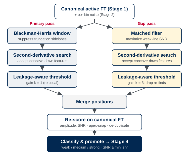
The Stage 3 detection workflow. The two passes run on separate apodizations and converge on the active FT, where amplitude and signal-to-noise are measured once for every peak.

Dual-pass detection

A single detector cannot meet both of Stage 3’s objectives. A strong line in a boxcar-truncated spectrum is surrounded by coherent truncation-leakage sidelobes — a sinc-like ripple skirt that an unapodized detector reads as a picket fence of spurious weak lines. Suppressing that ripple with a strong window function broadens every line and buries genuine weak lines next to strong ones. The two requirements are opposed, so Stage 3 runs two passes on two apodizations and merges the results.

The primary pass establishes robust strong-line positions. It transforms the active region through a Blackman-Harris window, which all but eliminates the truncation sidelobes, and locates peaks on the resulting magnitude spectrum. On the reference experiment this reduces the sidelobe-suspect detection fraction roughly five-fold. The apodization broadens the lines and loses some weak ones, which is acceptable: the primary pass need only return a clean, sidelobe-free list of the strong lines, which also seeds the second pass.

The gap pass recovers the weak lines the apodization smears away. It transforms the active region through the line’s matched filter — the time-domain envelope that maximizes signal-to-noise for a decaying line, \(e^{-t/\tau}\) for a Lorentzian instrument and \(e^{-(t/\tau)^2}\) for a Gaussian one. The decay constant \(\tau\) and the envelope shape both come from the Stage 2b calibration (its majority decay time, or the Gaussian twin when the line-shape vote recommends Gaussian); absent Stage 2b, the gap pass falls back to a 5 µs basis. Detections within a small exclusion radius of a primary peak are discarded as re-finds, so the gap pass contributes only new lines.

The matched filter is the optimal linear detector for a decaying line: it concentrates the line energy that an unweighted transform spreads across the skirt, so at a fixed false-positive load the gap pass recovers more real lines from fewer candidates. The matched-filter methods note derives this result and validates the recall. The gap pass is enabled by default (run_gap_pass=False / --no-gap-pass to disable).

Peak localization

Both passes localize peaks with the same operator: a Savitzky-Golay smoothed second-derivative search. It flags a peak only where the second derivative is negative (a genuinely concave-down feature) and retains the sharpest such points. This structural test is what makes the matched filter usable: a per-bin signal-to-noise threshold alone would accept every bin of a strong line’s monotonically decaying skirt, but those skirt bins are not concave-down maxima and are rejected, while true line centers are kept. The smoothing window spans about four line-widths, derived at run time from the grid spacing and the calibrated line-width (floored at five bins for polynomial stability); on the reference grid this reproduces the empirical eleven-bin primary-pass window.

Leakage-aware detection threshold

Neither pass masks a strong line’s leakage skirt, because the strong lines are themselves the source of the coherent leakage and a hard cutoff would delete them. Each pass instead raises its detection threshold continuously by the local coherent-leakage amplitude:

\[\text{threshold}(f) = \text{min\_snr}\cdot\sigma(f) + k \cdot \frac{S_\text{coh}(f)}{\sqrt{M}} \cdot \sigma(f).\]

The added term is the size of the coherent ripple at that frequency, measured by a complex-domain edge-coherence statistic \(S_\text{coh}\) over a band of \(M\) bins. A genuine line stands well above this floor; a strong line’s skirt ripple, which is that leakage, sits at it and is rejected. The statistic is computed on the de-ramped spectrum, which exposes the leakage rather than averaging it away under the active-region phase ramp.

The two passes require different gains \(k\) because they run on opposite-leakage spectra. The Blackman-Harris primary has already suppressed most of the leakage, so its floor is a small residual correction (primary_leakage_floor_k = 1). The matched-filter gap pass retains the full leakage, so its floor carries all of the suppression and needs a larger gain (gap_leakage_floor_k = 3). Both are per-instrument knobs; setting either to zero disables that floor.

Amplitude and signal-to-noise estimation

The two passes determine positions only. Every reported amplitude, signal-to-noise, and classification is re-measured on the single active FT (the unapodized, native-length spectrum that Stage 5 fits), so that all peaks share one signal-to-noise scale and the overlay matches the spectrum the fit sees. The apodized primary and matched-filter spectra are detection scaffolding; no apodized amplitude is ever reported.

Signal-to-noise is the magnitude’s excess over the local coherent-leakage pedestal, \((|X| - \text{pedestal})/\sigma\), not the raw \(|X|/\sigma\). The Stage 2 \(\sigma\) is the pedestal-subtracted fluctuation noise, so on a strong leakage pedestal — the limit where a dense forest of lines fills every quiet bin, several \(\sigma\) above the floor — the raw ratio would float every bin, genuine line or pure pedestal noise alike, above the cutoff and flood the later stages. The pedestal is the same per-bin coherent-leakage amplitude that raises the detection threshold; subtracting it scores the honest signal. A real line is sharp, so its own height is diluted across the coherence band and barely enters the pedestal, leaving its SNR essentially unchanged, while broad leakage is removed. The raw magnitude is still reported as the amplitude.

Re-measuring on the active grid also corrects two position artifacts. The second-derivative locator lands a few points off the true apex for ultra-narrow lines, so each detection is apex-snapped to the nearest local maximum on the scoring spectrum, recovering the correct peak height — without this, ultra-narrow lines under-report their amplitude by tens of percent. Detections that snap to the same grid point (split-strong-line artifacts, or a line found by both passes) are then de-duplicated, keeping the strongest.

Detection always runs on the Stage 1 active FT, including its frequency trim; there is no separate Stage 3 trim or zero-padding. Set the analysis band by running Stage 1 with the desired --trim beforehand.

Classification and promotion

Each peak is classified by signal-to-noise alone into weak, medium, or strong using two absolute boundaries (default 10 and 50). Absolute cutoffs are used rather than percentiles because the detected-peak SNR distribution is anchored at the detection floor with a heavy upper tail in every regime: across the reference fixtures, which span three orders of magnitude in line strength, all three tiers stay populated and the fixed boundaries generalize, where percentile boundaries would brand half of a sparse spectrum’s real lines weak. Only the strong tier drives the later stages: a strong line is a leakage source, so Stage 4 uses the strong tier to anchor its window grouping and to decide which lines are attached as fixed contributors to neighboring windows their skirts reach. The weak/medium distinction is curation and reporting labeling, carried for the analyst rather than consumed by an algorithm.

Detection and promotion are separated, which is what allows aggressive detection without flooding the later stages:

• The user-facing min_snr (default 3) is the promotion cutoff: the active-grid signal-to-noise at or above which a peak advances to Stage 4. The default sits at the cross-fixture knee where the candidate count transitions from noise-and-leakage structure to the real-line plateau.

• Detection itself runs at a fixed lower internal floor (2.0), independent of the promotion cutoff. Detecting at the promotion cutoff and then re-measuring on the active grid would lose lines that genuinely clear the cutoff there; detecting lower recovers them, and below the internal floor there is only noise. The floor is re-applied to the active-grid excess SNR after re-measurement: the apodized detection spectra flatten the leakage pedestal on their own grids, so a pedestal-noise bump can clear the floor there yet be pure pedestal on the active FT, and the second pass drops it before it is stored. Peaks between the internal floor and the promotion cutoff are kept (so the cutoff stays re-thresholdable); only sub-floor pedestal noise is discarded.

Each detected peak is persisted with a promoted flag derived from the stored cutoff, so re-thresholding is free and an edited list re-derives the flag cleanly.

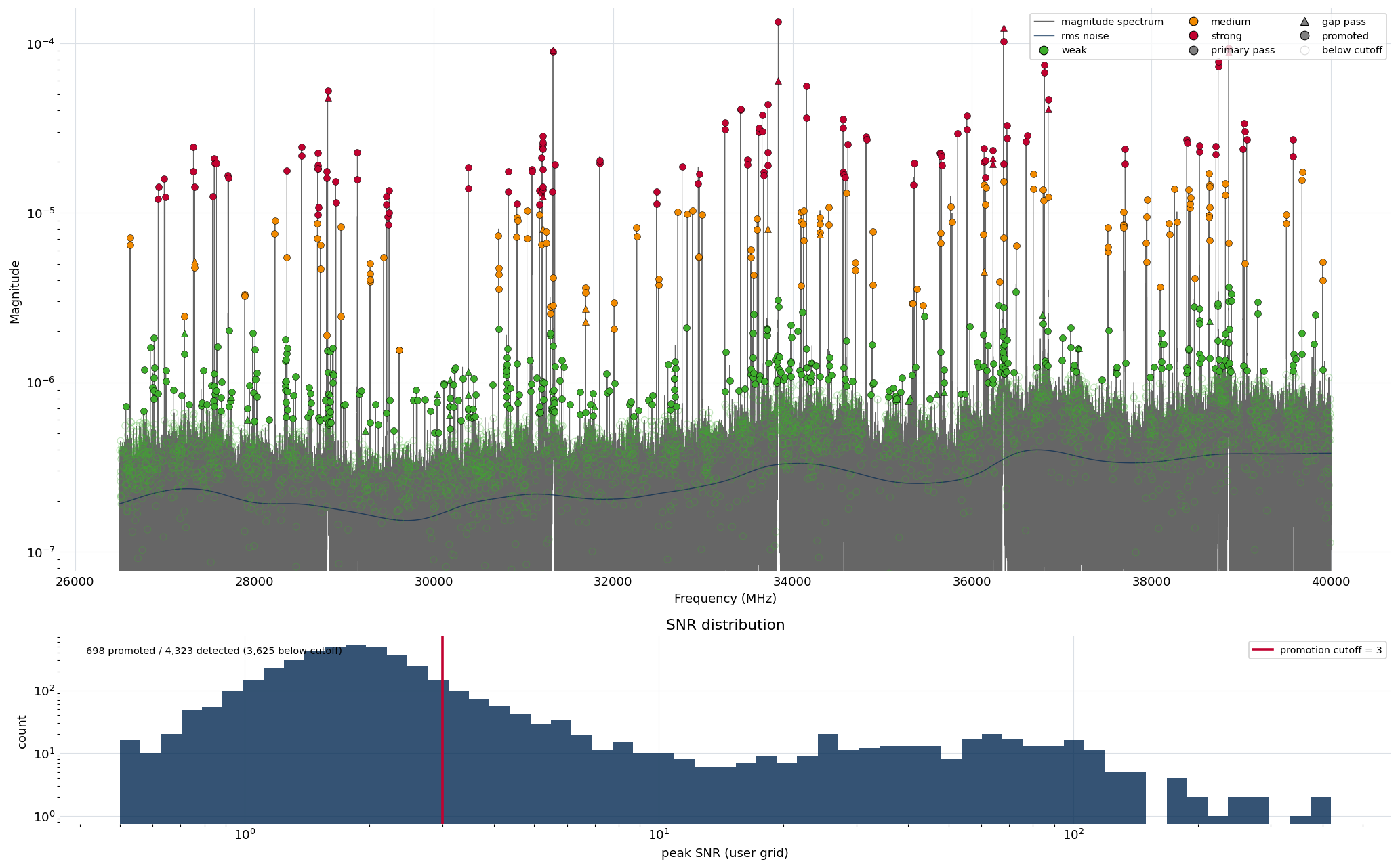
Stage 3 detection on the example experiment. Top: the classified peaks over the active spectrum (gray) and its per-bin noise, colored by SNR tier (green weak, orange medium, red strong), marker-styled by pass (circles primary, triangles gap), and filled when promoted or open when below the promotion cutoff. The log magnitude axis renders the noise floor and the hundreds-of-times stronger lines on one scale. Bottom: the curation panel, the signal-to-noise distribution of every detected peak with the promotion cutoff marked, used to set the threshold against the visible split between the near-noise hump and the real-line tail before peaks move to Stage 4.

Running the stage

Stage 3 requires Stages 1 and 2, and consumes Stage 2b when present:

$ ftmwpipeline peaks run exp_2638.ftmw
$ ftmwpipeline peaks show --snr-histogram exp_2638.ftmw

The same operations on the Python interfaces:

import ftmwpipeline.api as ftmw

peaks = ftmw.detect_peaks("exp_2638.ftmw")   # all detected peaks
ftmw.visualize_peaks("exp_2638.ftmw", show_snr_histogram=True)

# or, object-oriented
from ftmwpipeline import Pipeline
pipe = Pipeline.open("exp_2638.ftmw")
peaks = pipe.detect_peaks()
promoted = [p for p in peaks if p.properties["promoted"]]

detect_peaks returns the full candidate list (the curation substrate); Stage 4 consumes only the promoted subset. Re-running detection invalidates any Stage 4 window plan built on the old peaks.

The defaults are calibrated for the reference instrument and need no adjustment for routine use. The behavior is controlled by the knobs below, set with per-knob flags on peaks run (e.g. --min-snr), through a preset, or via settings=PeakDetectionSettings(...) on the Python interfaces; how explicit, preset, persisted, and recommended values resolve is described on Settings and presets.

Knob	Default	Role
min_snr	3	Promotion cutoff: the active-grid signal-to-noise at or above which a peak advances to Stage 4. The main detection control.
weak_medium_snr / medium_strong_snr	10 / 50	The SNR classification boundaries.
run_gap_pass	true	Run the matched-filter gap pass that recovers weak lines (--no-gap-pass to skip it).
primary_window	blackmanharris	The primary-pass apodization window (sidelobe suppression; affects positions only, never reported amplitude).
min_exclusion_mhz	0.0	Half-width around each primary peak that the gap pass treats as a re-find.
sg_window / sg_order	11 / 3	The primary-pass Savitzky-Golay smoothing window and polynomial order.

Advanced knobs flow through a preset or a settings bundle rather than per-flag: the internal detection floor (internal_min_snr), the leakage-floor gains (primary_leakage_floor_k, gap_leakage_floor_k), the detection-grid zero-padding (detection_zpf, gap_active_zpf), the grid-aware Savitzky-Golay rule (sg_fwhm_coverage, sg_min_window), and the scatter knobs for the primary pass’s own apodized-domain noise estimate. These rarely need touching.

Inspecting the result

peaks show overlays the classified peaks on the active spectrum on a log magnitude axis. Adding --snr-histogram appends the curation panel of the figure above (the signal-to-noise distribution of every detected peak with the promotion cutoff marked), the view for choosing a promotion threshold deliberately. By default the command opens an interactive window; --no-interactive together with -o saves a static image to the given path instead.

Curation and the handoff to Stage 4

Detection and window assignment are deliberately separate stages, so the detected-peak list is a curation point: an analyst can load it, add or remove peaks, adjust the promotion threshold, and re-save before windows are built. The peak list is persisted as a flat set of equal-length parallel arrays plus the detection parameters, an on-disk form built to edit. The loader validates the structure loudly: a missing column, mismatched lengths, or an unknown classification label raises an error rather than silently dropping data, so a malformed edit fails immediately rather than corrupting the fit.

The promoted peaks then drive two downstream consumers. Stage 4 builds the analysis windows from the promoted peaks, using the strong-line classification to decide which clusters need dedicated handling, and Stage 5 seeds its starting positions from the detected peaks within each window.

Limitations

• Detection deliberately smears close lines together where the primary pass’s apodization or the grid spacing cannot resolve them. This is by design (the per-window fit separates them) and means the Stage 3 count is a candidate count, not the final line count.

• The continuous leakage floor suppresses, but does not perfectly remove, the ripple at the skirts of the very strongest lines; a few near-skirt candidates can survive into the list, where the fit and the curation pass resolve them.

• Detection runs on the trimmed active band, so a line outside it is never seen. Set the band wide enough at Stage 1 to cover every region of interest.

With a classified, curated peak list in hand, Stage 4 groups the promoted peaks into the disjoint analysis windows the fit runs on.