Stage 2: Noise Estimation

Overview

Stage 2 measures the noise of the spectrum: a per-bin RMS amplitude \(\sigma_x(f)\) that quantifies how large a feature must be to stand above the noise. Every later stage divides by it — peak detection thresholds a signal-to-noise ratio against it, window assignment plans against it, and the fit weights its residuals by it — so the noise estimate is the statistical reference for the whole back half of the pipeline. The estimate is one value per frequency bin, because the noise on an FTMW instrument is not flat: it varies across the band with the receiver bandpass, the mixer and local-oscillator artifacts, and frequency-dependent amplifier noise.

The estimate is the per-bin complex RMS \(\sigma_x = \sigma_c\sqrt{2}\), where \(\sigma_c\) is the per-quadrature noise (the real and imaginary parts each carry \(\sigma_x^2/2\)). This is the convention the fit’s \(\chi^2\) weighting consumes.

Method

Stage 2 measures and stores the noise on the active FT — the transform of just the [start_us, end_us] active region, trimmed to the analysis band. This is the single grid every later stage scores, plans, and fits on (the full-record spectrum is a Stage 0/1 start-time comparison view only); it is rebuilt on demand from the persisted FID and the Stage 1 settings, so Stage 2 always measures on exactly the grid the downstream stages consume.

The obvious estimate, the magnitude level in the quiet regions between lines, fails on high signal-to-noise, line-dense spectra, because it measures a coherent leakage pedestal rather than the random noise. The scatter estimator instead isolates the white, bin-to-bin scatter of the magnitude from the smooth pedestal, yielding a per-bin \(\sigma_x(f)\) that follows the receiver noise while ignoring the lines on top of it. The two sections below detail the pedestal contamination and the estimator that defeats it.

Noise vs. leakage

The active FT is deliberately raw and unapodized. A boxcar transform of a strong line has a slowly decaying magnitude skirt, and the transform’s own sidelobes ring across the entire record. Any single line’s wings are small, but the sum of the far-wings of hundreds of strong lines forms a smooth pedestal that fills every quiet bin. A level-based estimator measures that pedestal, not the random noise.

The two are physically distinct: the random noise averages down with shot count as \(1/\sqrt{N}\), while the pedestal is proportional to the (coherently averaged) signal and is constant in \(N\). A level estimator therefore reads \(\sqrt{\sigma^2 + \mathrm{pedestal}^2}\) — it tracks the true noise at low signal-to-noise but plateaus at high signal-to-noise, over-reporting the noise by up to 6× on the most extreme fixtures. Because the error grows with signal-to-noise, no amount of better binning or line-trimming on the magnitude level can remove it; the quantity being measured is the wrong one.

Estimating noise from spectral scatter

The estimator (estimate_noise_scatter()) separates the noise from the pedestal with a high-pass along the frequency axis: the noise is the white, bin-to-bin scatter of the magnitude, while the pedestal is its smooth part. In outline:

1. Pedestal. Estimate the smooth leakage pedestal as a broad running median of the magnitude (width pedestal_mhz). Bins already flagged as lines are interpolated over first, so strong-line power does not pull the pedestal up near lines.

2. High-pass and self-mask. The residual |X| − pedestal is white where there is only noise. Bins whose residual exceeds line_k robust standard deviations are flagged as lines, and the mask is refined over n_iter passes. (Stage 2 runs before peak detection, so it cannot lean on a peak list — it finds the lines itself.)

3. Region-aware scatter → σ. In each sliding window_mhz region, take the robust scatter (a median absolute deviation) of the residual over the surviving non-line bins, and convert it to the underlying noise. Because the magnitude of a complex spectrum is Rician, the scatter-to-σ factor depends on the local regime (from strong-line-dominated to pure noise); with region_aware enabled, a calibrated lookup recovers the regime-correct factor from the spectrum itself.

4. Smooth. Interpolate the per-region σ across the band, then smooth it. Line skirts and sidelobes can only add to the local scatter, so the true noise floor is the lower envelope of the regional estimates: a broad moving median (smoothing_mhz) rides that floor straight through line-dense bands instead of bumping up under them, and a final Gaussian pass (convolve_mhz) removes the median’s staircase without re-inflating it.

The result is a smooth per-bin \(\sigma_x(f)\) that follows the real, slowly varying noise structure of the receiver while ignoring the lines that sit on top of it. Validation against shot-count scaling and frame-difference truth shows it stays close to the true noise across a \(10^3\)–\(10^6\) signal-to-noise range, where a naive level estimator over-reports by up to 6×; the derivation and validation are in Noise estimation at high signal-to-noise.

Running the stage

Stage 2 requires Stage 1. The command runs the estimator and stores the result:

$ ftmwpipeline noise run exp_2638.ftmw

The same operation on the Python interfaces:

import ftmwpipeline.api as ftmw
noise = ftmw.estimate_noise("exp_2638.ftmw")

# or, object-oriented
from ftmwpipeline import Pipeline
pipe = Pipeline.open("exp_2638.ftmw")
noise = pipe.estimate_noise()

The defaults are calibrated for the reference instrument and need no adjustment for routine use. The estimator’s behavior is controlled by the following knobs, set with per-knob flags on noise run (e.g. --window-mhz), through a preset, or via settings=NoiseSettings(...) on the Python interfaces; how explicit, preset, persisted, and recommended values resolve is described on Settings and presets.

Knob	Default	Role
window_mhz	80	Width of the per-region scatter window — the scale over which σ is taken to be locally constant.
pedestal_mhz	20	Running-median width that isolates the smooth leakage pedestal.
line_k	8	Robust-σ multiple above which a residual bin is flagged as a line and excluded.
n_iter	3	Self-mask refinement iterations.
region_aware	true	Use the region-aware Rician correction (otherwise a fixed mid-regime factor).
smoothing_mhz	800	Width of the broad lower-envelope median that rides the noise floor through line-dense bands (0 disables smoothing).
smoothing_percentile	50	Percentile of that smoothing (50 is the median; lower values give a more aggressive lower-envelope).
convolve_mhz	200	Gaussian width of the second, staircase-removing smoothing pass (0 disables it).

The Rician correction table and the \(\sigma_x = \sigma_c\sqrt{2}\) conversion are analytic and are not tunable.

Inspecting the estimate

noise show overlays the estimate on the active-FT magnitude spectrum — the spectrum, the bins kept as noise, and the per-bin σ with \(3\sigma\) and \(5\sigma\) reference levels:

$ ftmwpipeline noise show exp_2638.ftmw

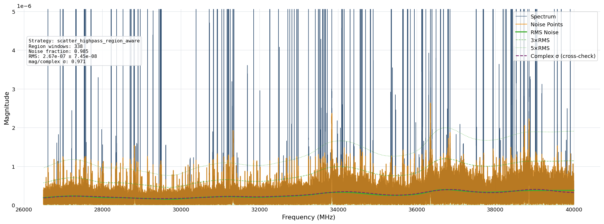
The scatter noise estimate on the example experiment, overlaid on the active-FT magnitude spectrum (clipped to the noise scale). The per-bin σ and its \(3\sigma\) / \(5\sigma\) levels ride through the line-dense regions rather than bulging beneath the lines.

The σ curve should track the receiver noise across the band and ride through the line-dense regions rather than bulging upward beneath the lines — the latter is the leakage-pedestal contamination the scatter estimator is designed to avoid. The same figure is available from Python through ftmwpipeline.api.visualize_noise() and Pipeline.visualize_noise.

The overlay marks many clearly visible lines among the bins kept for the estimate, rather than masking them out, which can look like it would inflate σ. It does not: the line self-mask is deliberately loose (line_k = 8) because the windowed scatter is a robust statistic that tolerates the line bins left in, and the broad lower-envelope median — not the mask — is what keeps line power out of σ. Why a tighter threshold would instead bias σ low, and why the loose mask’s only cost is a small weak-line floor, is analyzed in Choosing the line-mask threshold.

Complex-domain cross-check

The estimator works on the magnitude spectrum, where pure noise is Rayleigh-distributed and a small regime correction is needed to recover σ. As an independent guardrail, Stage 2 also computes σ directly from the real and imaginary parts over the same noise bins (for pure noise these are symmetric, zero-mean Gaussian, needing no regime correction) and records the ratio of the two estimates in the diagnostics (mag/complex σ on noise show, with the complex curve overlaid). The magnitude estimate normally sits a few percent below the complex one; a larger divergence is flagged with a warning, indicating the per-bin σ may be biased on that spectrum.

The stored per-bin σ is the input to Stage 3, which thresholds the signal-to-noise ratio of candidate peaks against it.