Timebase self-calibration

A spectrometer reports frequencies in units of its digitizer’s sample rate. When that digitizer is locked to the laboratory frequency standard, the rate is exact and the frequency axis needs no correction. When it free-runs, it samples at a rate that is slightly wrong by a fractional scale error \(\varepsilon\), and every measured frequency inherits that error in proportion to how far it sits from the receiver’s center — a tilt of the whole frequency axis, not a constant shift. On the reference instrument \(\varepsilon \approx 2\) parts per million, which is tens of kilohertz at the top of the band: the dominant accuracy term, far above the per-line fitting precision.

The error would be unrecoverable if the axis carried only molecular lines, whose true frequencies are the unknowns. It is recoverable because the spectrum also carries the instrument’s own clock tones (see Declaring Instrument Clocks). The Rb-locked tones sit at frequencies that are known exactly from clock arithmetic, so their measured offsets are direct samples of the same scale error. This note derives the estimator that reads those offsets — from each tone’s phase evolution, not from a fitted line width — bounds its precision, and validates it on a synthetic record with a known scale error and on the reference experiment. The figures and quoted numbers are regenerated by docs/source/methods/timebase_calibration/generate.py; see Reproducing this note.

The scale error stretches the frequency axis

A digitizer running at a fractional rate error \(\varepsilon\) measures a tone of true baseband frequency \(f_\text{bb}\) at

\[f_\text{meas} = (1 + \varepsilon)\, f_\text{bb}, \qquad \Delta f \equiv f_\text{meas} - f_\text{bb} = \varepsilon\, f_\text{bb}.\]

The offset \(\Delta f\) is linear in \(f_\text{bb}\) and passes through the origin: zero at the receiver center, largest at the far edge of the band. This is the signature the calibration exploits — not the size of any one offset, but that every tone’s offset falls on a single line through the origin whose slope is \(\varepsilon\). Because \(\varepsilon\) multiplies the baseband frequency, the absolute error grows across the band; at \(\varepsilon = 2\) ppm a tone \(16\) GHz above the receiver center reads about \(32\) kHz high.

Reading a tone’s offset from its phase

A clock tone does not decay: it is a continuous-wave sinusoid that persists across the whole acquisition. Its frequency is therefore most precisely read not from the width or position of a magnitude peak, but from how its phase advances in time. For a tone of nominal baseband frequency \(f_\text{bb}\), the calibration demodulates the raw record by multiplying it by \(e^{-2\pi i f_\text{bb} t}\). A tone exactly at its nominal frequency becomes a constant (DC) term; a tone offset by \(\delta f\) becomes a slow residual rotation,

\[z(t) = x(t)\, e^{-2\pi i f_\text{bb} t} \;\longrightarrow\; A\, e^{-2\pi i\, \delta f\, t},\]

a phase ramp whose constant slope is the offset. The calibration measures that slope by the maximum-likelihood estimate for a single tone: it block-averages the demodulated record and scans a fine grid of candidate offsets for the one whose complex sinusoid best correlates with the residual rotation — the peak of the coherent sum, refined by parabolic interpolation. No sinc or Lorentzian magnitude lineshape is ever fit.

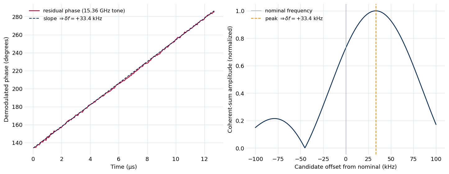
The measurement on the strongest clock tone of the reference experiment (15.36 GHz baseband). Left: after demodulating at the tone’s nominal frequency, the block-averaged phase advances linearly in time — a residual phase ramp whose slope is the frequency offset (the dashed line is that slope). Right: the coherent-sum amplitude against candidate offset; its sharp peak is the maximum-likelihood offset, here \(+33.4\) kHz. Both panels read the same offset from the tone’s phase evolution, with no lineshape fit.

Reading the offset from the phase evolution over the full acquisition time \(T\) is what makes it precise. The Cramer-Rao bound on a single-tone frequency estimate from \(N\) samples of signal-to-noise ratio \(\mathrm{SNR}\) is

\[\sigma_f \;=\; \frac{\sqrt{6}}{\pi}\,\frac{1}{T\,\mathrm{SNR}},\]

inversely proportional to the duration the phase is observed over, not to the linewidth. For the strong clock tones (\(\mathrm{SNR}\) in the thousands over a \(\sim 13\)-microsecond record) this is parts in \(10^{8}\) — orders of magnitude finer than reading the same tone’s position from its magnitude peak, whose width is set by \(1/T\) and whose centroid the noise perturbs at the bin scale.

From per-tone offsets to a shared ε

Each detected locked tone yields one offset \(\delta f_k\) at known baseband frequency \(f_k\), and one estimate \(\delta f_k / f_k\) of \(\varepsilon\). The consensus value is the weighted, shared-\(\varepsilon\) fit across all the tones — a line through the origin — with each tone weighted by its uncertainty,

\[\hat{\varepsilon} = \frac{\sum_k f_k\, \delta f_k / \sigma_k^2}{\sum_k f_k^2 / \sigma_k^2}, \qquad \sigma_{\hat{\varepsilon}} = \left( \sum_k \frac{f_k^2}{\sigma_k^2} \right)^{-1/2},\]

where \(\sigma_k^2 = \sigma_{f,k}^2 + (\kappa_\text{sys} f_k)^2\) adds a small per-tone systematic floor to the Cramer-Rao term. The high-frequency tones, whose offsets \(\varepsilon f_k\) are largest, carry the most leverage on the slope. Three properties make the fit robust:

• Out-of-band tones are the primary anchors. The strongest locked tones sit above the molecular band, where the chirp never excites and no line can pull the measurement. They are stable across the record and carry the longest lever arm on \(\varepsilon\).

• The drifting family identifies itself. A tone derived from the free-running digitizer sits at an exact rational frequency in sample space, so it does not share the common \(\varepsilon\) of the Rb-locked tones — it falls off the shared-\(\varepsilon\) line. A \(4\sigma\) consistency rejection, iterated to convergence, removes it (and any off-nominal tone) automatically. The same test that cleans the fit is the drifting-family discriminant.

• The scale error is per acquisition. \(\varepsilon\) is a property of one recording, not a fixed instrument constant, so the calibration is run and persisted per file. With every clock declared as locked it returns \(\varepsilon \approx 0\) — the expected null — and the axis needs no correction.

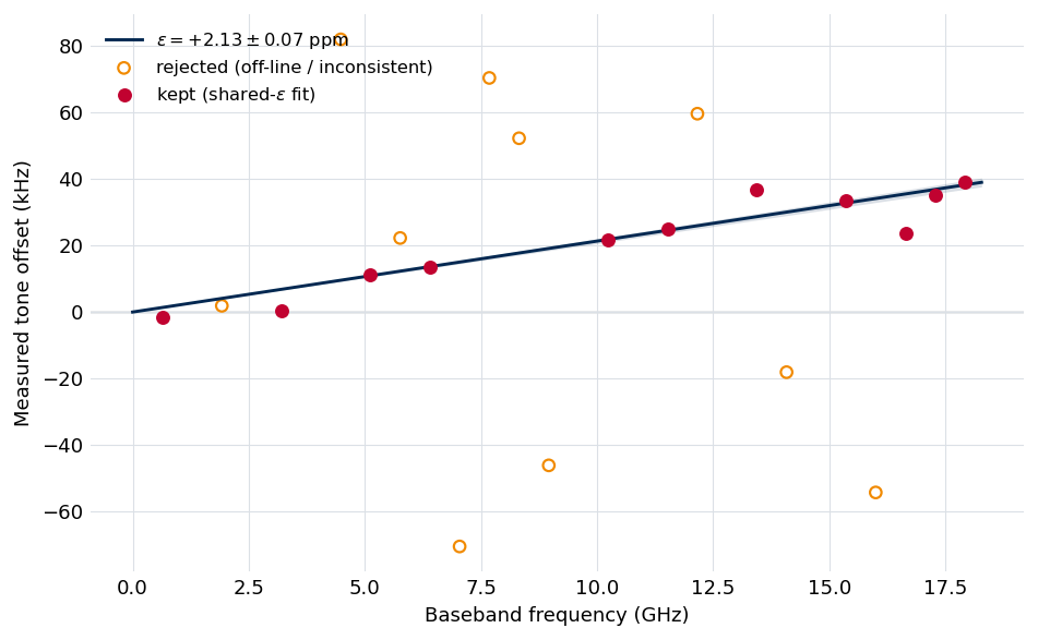
Timebase self-calibration on the reference experiment. Each point is one Rb-locked clock tone: its measured frequency offset against its baseband frequency. The kept tones fall on a straight line through the origin whose slope is the digitizer scale error \(\varepsilon\); a tone that does not share the common slope — inconsistent, off-nominal, or drifting — is rejected. The shaded band is the \(1\sigma\) uncertainty on the fitted \(\varepsilon\).

Validation

The estimator recovers a known scale error. A synthetic record planted with Rb-locked lattice tones at \(k\,g\,(1 + \varepsilon_\text{true})\) — together with a decaying off-lattice tone and an off-nominal spur carrying a fixed non-\(\varepsilon\) offset — is calibrated back to \(\varepsilon_\text{true} = 2.0\) ppm within \(0.01\) ppm, a small fraction of its \(0.09\) ppm formal uncertainty, and holds that recovery as the noise is raised through a factor of nine. The off-nominal tone is detected but rejected by the shared-\(\varepsilon\) consistency test, never entering the fit. With the systematic floor switched off, each kept tone’s reported uncertainty equals the Cramer-Rao bound \((\sqrt{6}/\pi)/(T\,\mathrm{SNR})\) to within rounding — the estimator is statistically efficient, not merely consistent.

On the reference experiment the three declared locked synthesizers gate a \(640\) MHz lattice; the calibration detects twenty-one tones on it, keeps the eleven that share a common slope, and rejects the ten that do not, returning

\[\varepsilon = +2.13 \pm 0.07 \;\text{ppm},\]

a measurement dominated by the out-of-band anchors near \(15\)–\(18\) GHz baseband. The strongest tone, at \(15.36\) GHz with a signal-to-noise ratio in the thousands, reads \(+33.4\) kHz high — the per-tone offset the figure above plots.

The estimator and its precision bound are validated here; the absolute accuracy of the corrected axis is the part still to be measured. A per-acquisition flat offset that the clock lattice cannot constrain (discussed below) sets a systematic floor that only an independent frequency reference can pin down. This page will gain that validation — a cross-instrument comparison against absolute references — as new experimental measurements become available.

How the correction reaches the line list

The calibration measures and persists \(\varepsilon\); it does not alter the spectrum. Stage 6 applies it when it consolidates the final-products table: each frequency is mapped back to the locked frame by \(f_\text{true} = f_\text{meas} / (1 + \varepsilon)\), and the calibration uncertainty enters the reported per-line budget as one of its three terms,

\[\sigma_f = \sqrt{\sigma_\text{stat}^2 + (\sigma_\varepsilon\, f_\text{bb})^2 + \sigma_\text{floor}^2}.\]

The pipeline reports precision, and treats a measured \(\varepsilon\) as a precision input: the scale error is determined from the data, so correcting it sharpens the axis without importing an external assumption. It does not silently assert an accuracy it cannot determine. A per-acquisition flat absolute offset remains — the down-conversion chain can shift the whole baseband comb by a constant the lattice cannot separate from a true common offset — so the systematic accuracy floor \(\sigma_\text{floor}\) defaults to zero and is the user’s declaration to make against an independent reference. The frequency-calibration state a report prints (absolutely calibrated, self-calibrated, or uncalibrated) is derived from the clock declaration and whether a timebase calibration was run. The Stage 6 page covers that budget in full.

Caveats

• Self-calibration fixes the slope, not the intercept. A measured \(\varepsilon\) removes the frequency-dependent stretch but leaves any per-acquisition constant offset; absolute accuracy needs an external reference, carried by \(\sigma_\text{floor}\).

• At least three consistent locked tones are required. The calibration reports a failed precondition when fewer survive the consistency fit, rather than returning an under-determined \(\varepsilon\).

• Instrument dependence. The lattice spacing and which tones fall in band are set by the declared clocks; the estimator and its Cramer-Rao bound are analytic and not tunable.

Reproducing this note

The figures and the quoted numbers are regenerated from the checked-in 2638 fixture under examples/blackchirp_data/ by:

python docs/source/methods/timebase_calibration/generate.py

which writes figures/*.png and results.json beside the script (a few seconds). Two fast, data-free invariants are exercised by the unit suite — the estimator recovers the planted \(\varepsilon\) and rejects the off-nominal tone, and each kept tone’s reported uncertainty matches the Cramer-Rao bound. The full fixture regeneration is guarded against drift by a slow-marked test that re-runs the harness and compares results.json within tolerance.