Stage 1: Fourier Transform

Overview

Stage 1 transforms the raw free-induction decay into the frequency-domain spectrum that every later stage works from. It selects the active region of the record, removes its DC offset, computes the discrete Fourier transform, maps the result onto molecular frequency, and restricts it to the analysis band. The settings that govern this transform are the experiment’s canonical FT settings: once stored, they bind the spectrum that noise estimation, peak detection, window assignment, and fitting all reproduce.

The transform yields a complex spectrum on a molecular-frequency axis in MHz. The spectrum is not stored in the .ftmw file; instead, Stage 1 persists the resolved settings, and the lightweight file model recomputes the spectrum on demand from the stored FID and those settings. Recomputation is deterministic, so any interface that opens the file reconstructs exactly the same spectrum. The file model, and what is stored versus recomputed, is described on Inside the .ftmw file.

Method

Stage 1 performs a fixed sequence of operations, none of which weights or interpolates the FID samples: the active region is selected and its DC offset removed, the discrete Fourier transform is taken at native length, the baseband axis is mapped to molecular frequency, and the spectrum is restricted to the analysis band (trim).

The transform is unconditionally unapodized, un-windowed, and native-length — no window function is applied to the FID, no exponential decay is multiplied in, and the record is not zero-padded. This is a deliberate choice. Apodization trades frequency resolution for lower sidelobes and biases the line shape, and zero-padding interpolates the spectrum between true bins, which corrupts the per-bin noise statistics that Stage 2 measures and the χ² statistics that the Stage 5 fit relies on. The robust per-window fit is the pipeline’s substitute for those conventional display-time treatments: it models the finite-acquisition line shape directly on the unmodified spectrum, so the FT is left faithful to the data.

The only operations performed on the FID are data selection and a baseline correction:

• Active-region selection (start_us / end_us) zeroes the record outside the chosen time window. The default start_us is the recommended start from Stage 0, which clears the excitation chirp and switch ring-down; an explicit value overrides it.

• DC removal subtracts the mean of the active region before the transform, suppressing the zero-frequency spike. This is automatic.

Molecular frequency and sideband

The transform is taken over the digitizer’s baseband frequencies, which are then mapped to molecular frequency using the probe frequency and the sideband recorded at import. For an upper-sideband measurement the molecular frequency is the probe frequency plus the baseband frequency; for a lower-sideband measurement it is the probe frequency minus the baseband frequency. The resulting axis is in MHz and increases with molecular frequency, so downstream stages and plots read directly in laboratory units.

Running the stage

The command computes the FT and stores the resolved settings as canonical:

$ ftmwpipeline ft run exp_2638.ftmw --trim 26500:40000

The same operation on the Python interfaces:

import ftmwpipeline.api as ftmw
ftmw.compute_ft("exp_2638.ftmw", trim=(26500, 40000))

# or, object-oriented
from ftmwpipeline import Pipeline
pipe = Pipeline.open("exp_2638.ftmw")
pipe.compute_ft(trim=(26500, 40000))

Because the FT is unapodized and native-length, the only parameters are the active-region bounds, the analysis band, and a display scale:

Parameter	CLI flag	Meaning
trim	--trim MIN:MAX	The analysis band in MHz, given as a colon-delimited range. The spectrum is restricted to this range, which is the active FT that later stages operate on. For the example experiment the active band is 26500:40000.
start_us	--start-us	Start of the active region in microseconds. Defaults to the Stage 0 recommended start.
end_us	--end-us	End of the active region in microseconds. Defaults to the end of the record.
units_power	--units-power	Power-of-ten display amplitude scale (6 for µV). Affects only the reported amplitudes, not the analysis.

The --trim range uses the same MIN:MAX form as the persisted settings and the whole-pipeline run command. How an explicit value resolves against a persisted or recommended one is described on Settings and presets.

Committing and re-running the transform

When the transform is run as a user action (the CLI ft run, or compute_ft() with explicit settings), the resolved settings (including the frequency trim) are written as the experiment’s canonical FT settings, and Stage 1 is marked complete. Every stage built on the spectrum reads back exactly these settings, so the noise estimate, the peak list, the window plan, and the fit are all defined against one spectrum.

Changing these settings therefore invalidates that downstream work. If ft run is repeated with settings that differ from the stored ones, the results that depend on the FT (Stage 2 noise and everything after it) are removed and a warning is logged, so they are recomputed against the new spectrum rather than silently mixed with stale results. Repeating the transform with identical settings changes nothing, which keeps re-running an import-and-FT cell in a notebook safe.

Inspecting the transform

ft show renders the complete FID-to-spectrum workflow (the raw FID with the active-region bounds marked, the preprocessed FID, and the magnitude and real/imaginary spectrum panels) for a set of parameters, without storing them. It is the tool for trying parameters before committing them with ft run:

$ ftmwpipeline ft show exp_2638.ftmw --start-us 2.0 --trim 26500:40000

The view is interactive by default; --no-interactive --output <path> writes a static image instead. Visualization never persists settings — once a choice looks right, re-run ft run with it to make it canonical.

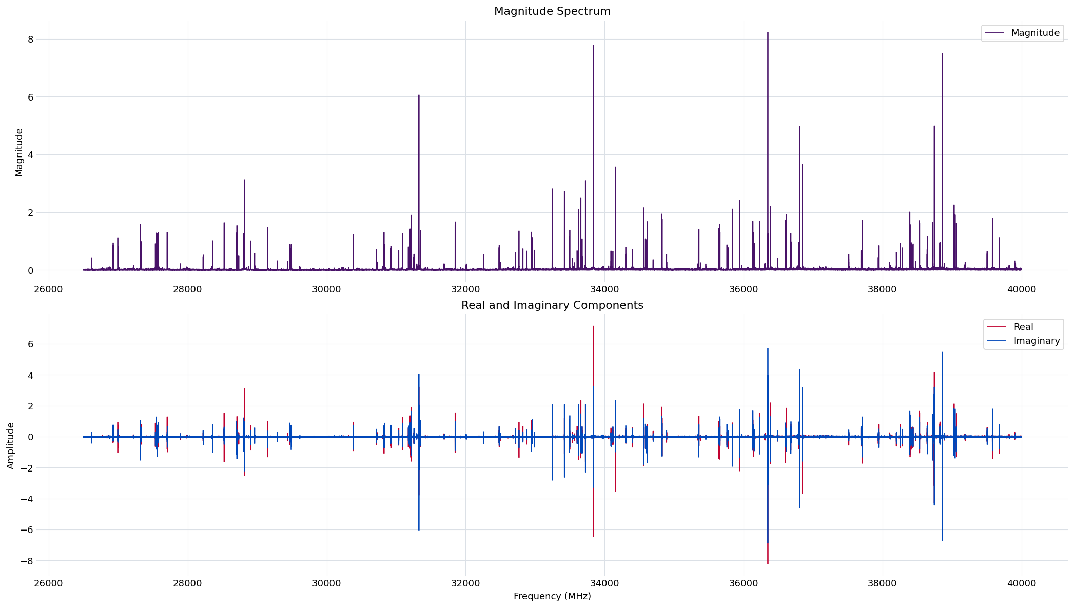
The active FT of the example experiment over the 26500:40000 MHz active band. Top: the magnitude spectrum. Bottom: the real and imaginary components on the same molecular-frequency axis. The transform is unapodized and native-length, so the line shapes and per-bin amplitudes are faithful to the data.

The resolved spectrum is the input to Stage 2, which measures the per-bin noise on the active FT.